- Author(s) of this documentation:
- Jacques-Olivier Lachaud and Bertrand Kerautret.
Part of the Topology package.
This part of the manual describes how to define digital objects. Subset of a digital sets are not really objects as long as they do not have some adjacency relation which describes how points (pixels in 2D, voxels in 3D, spels in nD) are connected. Digital topology was introduced by Rosenfeld as a framework to describe consistently how objects are connected and how complements of objects are connected. It has lead him to define two different adjacencies relations, one for the foreground (object), one for the background (complement of object). For well chosen adjacency relations, we find again some classical results of topology in continuous domains. For instance, the Jordan property may hold for several couples of adjacencies.
The topology kernel of DGtal allows to define adjacencies, topologies, objects, and operations with objects in a very generic framework. Some of these operations have been specialized for standard spaces and topologies, in order to keep operations as fast as possible.
Once a topology (class DigitalTopology) has been defined from two adjacencies (models of concepts::CAdjacency), a digital object (class Object) has a border which is the set of elements adjacent to its complement. The border is again a digital object. A digital object can also be seen as a graph, which can be traversed in many ways, although the breadth-first is often very useful (class Expander).
Adjacency relations
An adjacency relation in a digital space X describes which points of the digital space are close to each other. Generally it is a reflexive and symmetric relation over the points of X. Interested readers can read the works of Azriel Rosenfeld and Gabor Herman to see a well-founded theory of digital spaces.
4- and 8- adjacencies in Z2
In \( Z^2 \), two adjacencies are used. The so-called 4-adjacency tells that a 2D point is adjacent to itself and to four other points (north, east, south, and west points). The so-called 8-adjacency tells that a 2D point is adjacent to itself and to eight other points (the four points of the 4-adjacency relation added with four points in the diagonals). These two adjacencies relations are translation invariant, symmetric, reflexive. You can define them as follows with DGtal:
You can equivalently use the types Z2i::Adj4 and Z2i::Adj8, (namespace Z2i in "DGtal/helpers/StdDefs.h"), defined on SpaceND<2,int>.
It is well known that if you choose the 4-adjacency for an object, one should choose the 8-adjacency for the background in order to get consistent topological properties. For instance a simple 4-connected digital close curve (of more than 4 points) splits the digital space into two 8-connected background components (digital Jordan theorem). The same is true if you choose the 8-adjacency relation for the object, the 4-adjacency should be choosed for the background. This is called the digital Jordan theorem (Rosenfeld).
6-, 18- and 26- adjacencies in Z3
Similarly as the 4-,8- adjacencies in 3D, the name of the 6-, 18-, 26- adjacencies defined in Z3 comes from the number of proper adjacent points for each point. Seeing a digital 3D point as a cube, the 6-neighbors are the points sharing at least a face with the cube, the 18-neighbors are the ones sharing at least an edge, while the 26-neighbors are the ones sharing at least a vertex. These three adjacencies relations are translation invariant, symmetric, reflexive. You can define them as follows with DGtal:
You can equivalently use the types Z3i::Adj6, Z3i::Adj18 and Z3i::Adj26, (namespace Z3i in "DGtal/helpers/StdDefs.h"), defined on SpaceND<3,int>.
Metric adjacencies in Zn
Adjacencies based on metrics can be defined in arbitrary dimension. They all have the properties to be translation invariant, reflexive and symmetric. They include the standard 4-, 8-adjacencies in Z2 and 6-, 18-, and 26-adjacencies in Z3. Given a maximal 1-norm n1, two points p1 and p2 are adjacent if and only if \( \| p2 - p1 \|_1 \le n1 \) and \( \| p2 - p1
\|_\infty \le 1 \). Metric adjacencies are implemented in the template class MetricAdjacency. For now, only metric adjacencies in Z2 are specialized, so as to be (slightly) optimized.
Concepts CAdjacency et CDomainAdjacency
Adjacencies are used at many places as a basis for more complex operations. To keep genericity and efficiency, adjacencies should satisfy the concept concepts::CAdjacency. They are specialized only at instanciation as argument to templates. A model of concepts::CAdjacency should define the following inner types:
- Space: the space of the adjacency.
- Point: the digital point type.
- Adjacency: the type of the adjacency itself.
It should also define the following methods:
- isAdjacentTo
- isProperlyAdjacentTo
- writeNeighborhood
- writeProperNeighborhood
Methods writeNeighborhood and writeProperNeighborhood are overloaded so as to substitute their own predicate with another user-given predicate. They are useful to restrict neighborhoods.
A concepts::CDomainAdjacency refines a concepts::CAdjacency by specifying a limiting domain for the adjacency. It adds the following inner types:
- Domain: the type of embedding domain.
- Predicate: the type of the predicate "is in domain ?".
It should also define the following methods:
- domain
- predicate
Digital topology over a digital space
A digital topology is a couple of adjacencies, one for the foreground, one for the background. The template class DigitalTopology can be used to create such a couple.
The following lines of code creates the classical (6,18) topology over \( Z^3 \).
The foreground adjacency is classically called kappa \( \kappa \) while the background is called lambda \( \lambda \) . Any topology has a reversed topology which is the topology \( (\lambda,\kappa) \).
A topology can be a Jordan couple. In this case, some objects of this space have nice properties. The reader is referred to the papers of Herman or to its book Geometry of digital spaces .
Digital objects
A digital object is a set of points together with a topology describing how points are close to each others. In DGtal, they are defined by the template class Object, parameterized by the topology (a DigitalTopology) and a digital set of points (any model of CDigitalSet like DigitalSetBySTLSet or DigitalSetBySTLVector).
The digital object stores its own set of points with a copy-on-write smart pointer. This means that a digital object can be copied without overhead, and may for instance be passed by value or returned. The input digital set given at construction specifies the domain of the object, which remains the same for the lifetime of the object.
Construction of digital objects
A digital object is generally initialized with some given set. The type of the set can be chosen so as to leave to the user the choice of the best set container for the object. You may use the DigitalSetSelector to let the compiler choose your digital set container at compilation time according to some preferences. The choice DigitalSetBySTLSet is the most versatile and generally the most efficient. The choice DigitalSetBySTLVector is only good for very small objects.
Objects may also be initialized empty, so that you can easily use a container to store them. Of course, they are not valid in this case.
Neighborhood of a point in an object
An object proposes several methods to return the neighborhood of a given point of the object.
- Object::neighborhood, Object::properNeighborhood: the neighborhoods are returned as objects (with a digital set type considered small).
- Object::neighborhoodSize, Object::properNeighborhoodSize: prefer these methods if you only need the cardinal of the neighborhoods and not the neighborhoods itselves
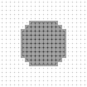
Border of a digital object
Objects have a border, which are the points which touch the complement in the sense of background adjacency. A border of an object is itself an object, with the same topology as the object.
The resulting border can be visualized for instance by: (see 3dBorderExtraction.cpp)
see example 3dBorderExtraction.cpp
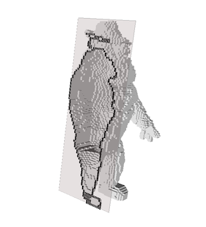
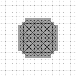
see example: 3dBorderExtractionImg.cpp
Connectedness and connected components
The digital topology induces a connectedness relation on the object (transitive closure of the foreground adjacency) and a connectedness relation on the complement of the set (transitive closure of the background adjacency). Objects may be connected or not. The connectedness is stored with the object, if it is known. The method Object::connectedness returns CONNECTED, DISCONNECTED or UNKNOWN depending on the connectedness of this object and if it has been computed. The method Object::computeConnectedness forces the computation. After this process, the connectedness is either CONNECTED or DISCONNECTED.
Furthermore, you can use the method Object::writeComponents to compute all the connected components of this object. It also updates the connectedness of this object to either CONNECTED or DISCONNECTED depending on the number of connected components. Each connected component is of course CONNECTED.
You may use writeComponents as follows:
You must be careful when using an output iterator writing in the same container as 'this' object (see Object::writeComponents).
Simple points
A basic mechanism for simple points is implemented in the Object class. It relies on the well-known definition of simple points of [14] , based on the number of connected components in a geodesic neighborhood of the point. It is valid in 2D and 3D. It should not be sufficient in nD, since toric connected components may appear. However, you can use it anyway as a kind of "extended" simplicity.
To test if a point is simple for an object, just call the method Object::isSimple with the point as parameter. To illustrate this, we give the full code for the homotopic thinning of a shape in 2D and 3D.
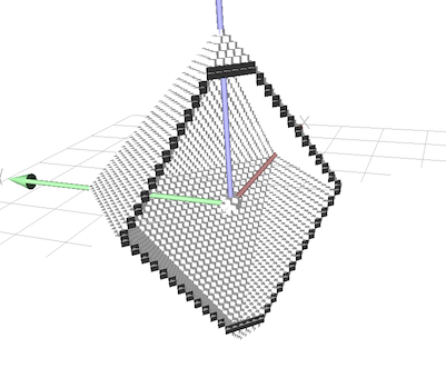
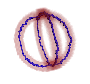
The file homotopicThinning3D.cpp illustrates the homotopic thinning on a 26_6 object.
First a digital object (with 6_26 adjacency) is defined from a digital set representing two rings :
Then the thinning is performed by testing if a point is simple:
Finally the result can simply be displayed using PolyscopeViewer:
We obtain the following result:
Neighborhood configurations, predicates and look up tables.
Object::isSimple(input_point) is an example of a predicate (ie. a function returning a Boolean value) that depends on the topology of the object and on the occupancy configuration of the input_point neighborhood.
There is a limited amount of possible configuration of the neighborhood depending on the dimension of the space. In 2D, there are 2^8 different neighborhood configurations, and in 3D 2^26. The result of the predicate will vary depending on the topology of the space, but the number of occupancy configurations will be the same for any topology in that dimension.
The calculation of a predicate for each point is repetitive and can be computationally intensive. However thanks to the limited amount of neighborhood occupancy configurations, we can pre-compute the Boolean result of the predicate for each configuration and store it in a look up table.
In DGtal, pre-computed look up tables for different predicates and topologies are distributed with the source code, and decompressed at build/install time to be ready to use. The tables locations are stored in string variables in: "DGtal/topology/tables/NeighborhoodTables.h"
Different functions to work with these pre-computed tables are in the header: "DGtal/topology/NeighborhoodConfigurations.h"
Object is able to take advantage of this just preloading the table before calling isSimple. This speeds up a thinning process by orders of magnitude.
In 2D:
- Note
- Be sure to choose the table with the same topology than the object.