Table of Contents
- Author(s) of this documentation:
- Jacques-Olivier Lachaud
- Since
- 1.1
Part of the Geometry package.
This part of the manual describes how to define and check digital convexity, in such a way that digital convex set are digitally connected.
The following programs are related to this documentation: geometry/curves/exampleDigitalConvexity.cpp, geometry/curves/exampleRationalConvexity.cpp, testBoundedLatticePolytope.cpp, testCellGeometry.cpp, testDigitalConvexity.cpp
Introduction to digital convexity
The usual definition for digital convexity is as follows. For some digital set \( S \subset \mathbb{Z}^d \), \( S \) is said to be digitally convex whenever \( \mathrm{Conv}(S) \cap \mathbb{Z}^d = S \). Otherwise said, the convex hull of all the digital points contains exactly these digital points and no other.
Although handy and easy to check, this definition lacks many properties related to (continuous) convexity in the Euclidean plane.
We extend this definition as follows. Let \( C^d \) be the usual regular cubical complex induced by the lattice \( \mathbb{Z}^d \), and let \( C^d_k \) be its k-cells, for \( 0 \le k \le d \). We have that the 0-cells of \( C^d_0 \) are exactly the lattice points, the 1-cells of \( C^d_1 \) are the open unit segment joining 2 neighboring lattice points, etc.
Finally, for an arbitrary subset \( Y \subset \mathbb{R}^d \), we denote by \( C^d_k \lbrack Y \rbrack \) the set of k-cells of \( C^d \) whose closure have a non-empty intersection with \( Y \), i.e. \( C^d_k \lbrack Y \rbrack := \{ c \in C^d_k,~\text{s.t.}~ \bar{c} \cap Y \neq \emptyset \} \).
A digital set \( S \subset \mathbb{Z}^d \) is said to be digitally k- convex whenever \( C^d_k \lbrack \mathrm{Conv}(S) \rbrack = C^d_k \lbrack S \rbrack \). \( S \) is said to be fully (digitally) convex whenever it is digitally k- convex for \( 0 \le k \le d \).
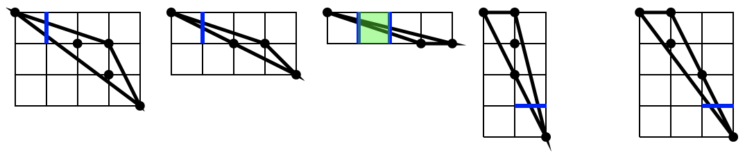
A fully convex set is always \( 3^d-1 \)-connected (i.e. 8-connected in 2D, 26-connected in 3D). Furthermore its axis-aligned slices are connected (with the same kind of connectedness). It is also clear that digitally 0-convexity is the usual digital convexity.
A last useful notion is the subconvexity. Let \( X \subset \mathbb{Z}^d \) some arbitrary digital set. Then the digital set \( S \subset \mathbb{Z}^d \) is said to be digitally k- subconvex to \( X \) whenever \( C^d_k \lbrack \mathrm{Conv}(S) \rbrack \subset C^d_k \lbrack X \rbrack \). And \( S \) is said to be fully (digitally) subconvex to \( X \) whenever it is digitally k- subconvex to \( X \) for \( 0 \le k \le d \).
Subconvexity is a useful for notion for digital contour and surface analysis. It tells which subsets of these digital sets are tangent to them.
Checking digital convexity
Three classes help to check digital convexity.
- BoundedLatticePolytope is the class that is used to build polytopes, i.e. intersections of half-spaces, which are a way to represent convex polyhedra.
- CellGeometry is used to store sets of cells and provides methods to build the set of cells that intersect a polytope or the set of cells that touch a set of digital points.
- DigitalConvexity provides many helper methods to build BoundedLatticePolytope and CellGeometry objects and to check digital convexity and subconvexity.
Lattice polytopes
For now, the class is quite limited. You may build a polytope in dimension \( d \le 3 \) from a range of \( n \le d + 1 \) points in general position. The polytope is then a simplex. For dimensions higher than 3, you may only builds the polytope from a full dimensional simplex, i.e. \( n = d + 1 \) in general position. Alternatively, you may provide a domain and a range of half-spaces to create the polytope.
You may also cut a polytope by a new halfspace (BoundedLatticePolytope::cut), count the number of lattice points inside, interior or on the boundary (BoundedLatticePolytope::count, BoundedLatticePolytope::countInterior, BoundedLatticePolytope::countBoundary) or enumerate them.
- Note
- Lattice point counting is done here in a naive way, by domain enumeration and constraint check. If m is the number of constraints and n the number of lattice points in the polytope domain, then complexity is in \( O(mn) \).
Last, you may compute Minkowski sums of a polytope with axis-aligned segments, squares or (hyper)-cubes (BoundedLatticePolytope::operator+=).
- Note
- You can check if the result of a Minkowski sum will be valid by calling BoundedLatticePolytope::canBeSummed before. The support is for now limited to polytopes built as simplices in 2D and 3D.
- See also
- DigitalConvexity::makeSimplex
Point check services:
- BoundedLatticePolytope::isInside checks if some point belongs to the polytope.
- BoundedLatticePolytope::isDomainPointInside checks if some point within the polyyope bounding box belongs to the polytope.
- BoundedLatticePolytope::isInterior checks if some point is strictly inside the polytope.
- BoundedLatticePolytope::isBoundary checks if some point is lying on the polytope boundary.
Standard polytope services:
- BoundedLatticePolytope::interiorPolytope returns the corresponding interior polytope by making strict every constraint
- BoundedLatticePolytope::cut cuts the polytope by the given half-space constraint
- BoundedLatticePolytope::swap swaps this polytope with another one in constant time
- BoundedLatticePolytope::operator*= dilates this polytope by a given factor
- BoundedLatticePolytope::operator+= performs Minkowski sum with some axis aligned unit segment/cell
Enumeration services:
- BoundedLatticePolytope::count counts the number of lattice points in the polytope
- BoundedLatticePolytope::countInterior counts the number of lattice points strictly inside the polytope
- BoundedLatticePolytope::countBoundary counts the number of lattice points on the boundary of the polytope
- BoundedLatticePolytope::countWithin counts the number of lattice points in some subdomain of the polytope
- BoundedLatticePolytope::countUpTo counts the number of lattice points in the polytope up to some maximal number
Lattice point retrieval services:
- BoundedLatticePolytope::getPoints outputs the lattice points in the polytope
- BoundedLatticePolytope::getInteriorPoints outputs the lattice points in the interior of the polytope
- BoundedLatticePolytope::getBoundaryPoints outputs the lattice points on the boundary of the polytope
- BoundedLatticePolytope::insertPoints inserts the lattice points in the polytope into some point set
Building a set of lattice cells from digital points
The class CellGeometry can compute and store set of lattice cells of different dimensions. You specify at construction a Khalimsky space (any model of concepts::CCellularGridSpaceND), as well as the dimensions of the cells you are interested in. Internally it uses a variant of unordered set of points (see UnorderedSetByBlock) to store the lattice cells in a compact manner.
Then you may add cells that touch a range of points, or cells intersected by a polytope, or cells belonging to another CellGeometry object.
- CellGeometry::addCellsTouchingPoints: Updates the cell cover with the cells touching a range of digital points [itB, itE).
- CellGeometry::addCellsTouchingPointels: Updates the cell cover with the cells touching a range of digital pointels [itB, itE).
- CellGeometry::addCellsTouchingPolytopePoints: Updates the cell cover with the cells touching the points of a polytope.
- CellGeometry::addCellsTouchingPolytope: Updates the cell cover with all the cells touching the polytope (all cells whose closure have a non empty intersection with the polytope).
- CellGeometry::operator+=( const CellGeometry& other ): Adds the cells of dimension k of object other, for
minCellDim() <= k <= maxCellDim(), to this cell geometry.
With respect to full digital convexity, CellGeometry::addCellsTouchingPolytope is very important since it allows to compute \( C^d_k \lbrack P \rbrack \) for an arbitrary polytope \( P \) and for any \( k \).
Checking digital (sub-)convexity
Class DigitalConvexity is a helper class to build polytopes from digital sets and to check digital k-convexity. It provides methods for checking if a simplex is full dimensional, building the corresponding polytope, methods for getting the lattice points in a polytope, computing the cells touching lattice points or touching a polytope, and a set of methods to check k-convexity or k-subconvexity.
Simplex services:
- DigitalConvexity::makeSimplex builds a simplex from lattice point iterators or initializer list
- DigitalConvexity::isSimplexFullDimensional checks that the given points form a full dimensional simplex
- DigitalConvexity::simplexType returns the simplex type in SimplexType::INVALID (when the number of points is less than d+1), SimplexType::DEGENERATED when it is not full dimensional, SimplexType::UNITARY when it is full dimensional and of determinant 1, SimplexType::COMMON otherwise.
- DigitalConvexity::displaySimplex outputs simplex information for debugging
Polytope services:
- DigitalConvexity::insidePoints returns the range of lattice points in the given polytope
- DigitalConvexity::interiorPoints returns the range of lattice points in the interior of the given polytope
Lattice cell geometry services:
- DigitalConvexity::makeCellCover either returns the lattice cells touching the given range of points or the lattice cells touching the given polytope
Convexity services:
- DigitalConvexity::isKConvex tells if a given polytope is k-convex
- DigitalConvexity::isFullyConvex tells if a given polytope is fully convex
- DigitalConvexity::isKSubconvex tells if a given polytope is k-subconvex to some cell cover
- DigitalConvexity::isFullySubconvex tells if a given polytope is fully subconvex to some cell cover
Rational polytopes
You can also create bounded rational polytopes, i.e. polytopes with vertices with rational coordinates, with class BoundedRationalPolytope. You must give a common denominator for all rational coordinates.
Then the interface of BoundedRationalPolytope is almost the same as the one of BoundedLatticePolytope (see Lattice polytopes ).
The classs BoundedRationalPolytope offers dilatation by an arbitrary rational, e.g. as follows
You may also check digital convexity and compute cell covers with bounded rational polytopes, exactly in the same way as with BoundedLatticePolytope.
- Note
- Big denominators increase with the same factor coefficients of half space constraints, hence the integer type should be chosen accordingly.
Further notes
The class BoundedLatticePolytope is different from the class LatticePolytope2D for the following two reasons:
- the class LatticePolytope2D is limited to 2D
- the class LatticePolytope2D is a vertex representation (or V-representation) of a polytope while the class BoundedLatticePolytope is a half-space representation (or H-representation) of a polytope.
There are no simple conversion from one to the other. Class LatticePolytope2D is optimized for cuts and lattice points enumeration, and is very specific to 2D. Class BoundedLatticePolytope is less optimized than the previous one but works in nD and provides Minkowski sum and dilation services.