3D Parametric Curves

Here we consider curves defined by parametric equations i.e., a group of functions of one variable, and hereafter called parametric curves. Each coordinate of a parametric curve, for a given parameter $ t $, is given by a corresponding function e.g., a parametric equation of a circle is given as $ \gamma : t \mapsto ( cos (t), sin(t) ) $. This module is related to digitization of 3D parametric curves.

In DGtal, each 3D parametric curve must be a model of C3DParametricCurve to be digitized.

Digitization - The algorithm

In this section we describe how to digitize 3D parametric curves using naive digitization method. Note that, the name of the method reflects the fact that this is a very naive method, which simply samples a curve with a given step parameter, and it is a numerical method that does not have any solid theoretical basis rooted in digital geometry. But in comparison to other known methods, that generate 26-connected digital curves, it does not require the coordinates' functions to be re-parametrized by each other, which often would involve existence of inverses of such functions. Such inverses even when they exist can be difficult to find.

In short the algorithm implemented in NaiveParametricCurveDigitizer3D.h is as follows.

Input: a 3D parametric curve $ \gamma $ (model of C3DParametricCurve), sampling step $ t $, and a sampling interval $ [t_{min}, t_{max}] $ such that $ t \in [t_{min}, t_{max}] $. Optionally, the user may provide a search parameter $ K_{NEXT} > 0 $ that controls how 26-adjacent neighbors are found. By default $ K_{NEXT} = 5 $.

Output: A sequence of integer points, which connectivity, in some places, may depends on $ K_{NEXT}, t $ and the relation between the curve's curvature and the digital grid (see some examples below).

Simplified pseudo-code:

Create a raw digitization
while $ t \in [t_{min}, t_{tmax}] $ do

point = [ $ \gamma(t) $] // [.] stands for a rounding function
weights[point] = weights[point] + 1
if not buffer.hasElement(point) then

buffer.push_back(point)

t = t + step

digital_curve.push_back(buffer[0])
Refine the digitization by keeping only the most meaningful points i.e., points of high coverage of $ \gamma $.
for $i = 1$ while $ i <$ size(buffer) do

for $ j = i + 1 $ and $ k = 0 $ while $ j <$ size(buffer) and $ k < K_{NEXT} $ do

if is26Connected(digital_curve.back(), buffer[j]) and weights[buffer[j]] $ > $ weights[buffer[i]] then

$ i = j $
$k = 0 $

else

$ k = k + 1 $

$ j = j + 1 $

digital_curve.push_back(buffer[i])
$ i = i + 1 $

Due to the weights fluctuations or curve behaviour we can still have points that should be removed to ensure 26-connectivity.
for $ i = 0 $ while $ i <$ size(buffer) do

$ tmp = i + 1 $
for $ j = i + 1 $ and $ k = 0 $ while $ j <$ size(buffer) and $ k < K_{NEXT} $ do

if is26Connected(digital_curve[i], digital_curve[j]) then

$ tmp = j $
$ k = 0 $

else

$ k = k + 1 $

$ j = j + 1 $

digital_curve.erase(i + 1, tmp)
$ i = tmp + 1 $

In the implemented version the buffer has size three times the value of $ K_{NEXT} $, and each time the buffer is flushed a part of the digital curve is created (see the two first nested loops in the code above). Also, the implemented version can treat closed curves and collect useful metadata.

Additional Information

The digitization implemented in NaiveParametricCurveDigitizer3D can collect, for each point of the output digital curve, information like

weights i.e., the point importance
time - a time value that minimize the distance between the integer point and $ \gamma $ for a given time step.

Note that, the time information is not computed by default therefore if not needed the user should avoid calling NaiveParametricCurveDigitizer3D::digitize(back_inserter_iterator, back_inserter_iterator), and use NaiveParametricCurveDigitizer3D::digitize(back_inserter_iterator), instead.

Examples

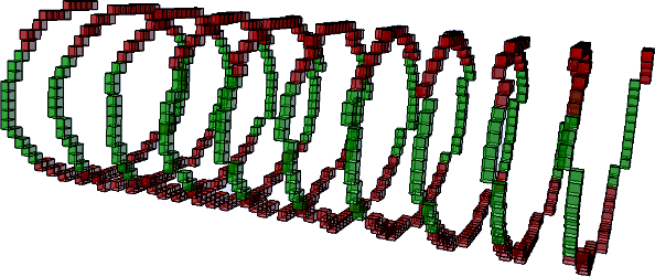
Example below shows how to digitize an elliptic helix (see EllipticHelix.h).

Before using NaiveParametricCurveDigitizer3D, you must include the following headers:

#include "DGtal/geometry/curves/parametric/EllipticHelix.h"

#include "DGtal/geometry/curves/parametric/NaiveParametricCurveDigitizer3D.h"

Note that, EllipticHelix.h should be replaced with the desirable curve. The list of 3D parametric curves is given below. Note that, EllipticHelix is the only curve that implements inverse functions (see EllipticHelix.h) for more information.

Then, you can construct the needed types as follows:

 typedef EllipticHelix < Space > MyHelix;
 typedef NaiveParametricCurveDigitizer3D < MyHelix >  DigitizerHelix;
 typedef NaiveParametricCurveDigitizer3D < MyHelix >::DigitalCurve MyDigitalCurve;
 typedef NaiveParametricCurveDigitizer3D < MyHelix >::MetaData MyMetaData;

Also, we can state instances of the digitizer and the curve:

 MyDigitalCurve digitalCurve;
 MyMetaData metaData;
 MyHelix helix( 15, 10, 1 );
 DigitizerHelix digitize;
 digitize.init ( M_PI / 2., ( MyHelix::getPeriod() * 10. ) + M_PI / 2., 0.0001 );
 digitize.attach ( &helix );

Finally, we can compute a digitization together with the meta information by calling:

digitize.digitize( back_insert_iterator < MyDigitalCurve> ( digitalCurve ), back_insert_iterator < MyMetaData > ( metaData ) );

The meta information can be then used, for example, to find main axis:

 for ( unsigned int i = 0; i < digitalCurve.size ( ); i++ )
 {
  if ( findMainAxis ( helix, metaData.at ( i ).first ) == 0 )
   viewer.setFillColor ( Color ( 255, 0, 0, 128 ) );
  if ( findMainAxis ( helix, metaData.at ( i ).first ) == 1 )
   viewer.setFillColor ( Color ( 0, 255, 0, 128 ) );
  if ( findMainAxis ( helix, metaData.at ( i ).first ) == 2 )
   viewer.setFillColor ( Color ( 0, 0, 255, 128 ) );
  viewer << SetMode3D ( digitalCurve.at ( i ).className ( ), "PavingWired" ) << digitalCurve.at ( i );
 }

See exampleParamCurve3dDigitization.cpp and exampleTrofoliKnot.cpp

Implemented Curves

Elliptic Helix (see EllipticHelix.h)

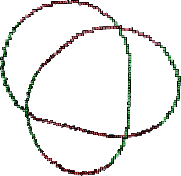
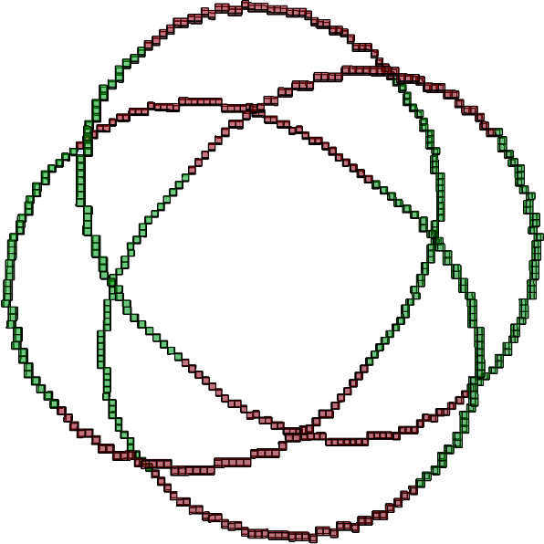
Knot $ 3_1 $ (see Knot_3_1.h)

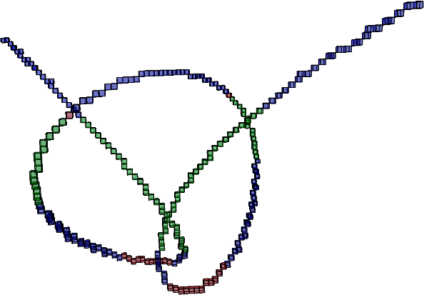
Knot $ 3_2 $ (see Knot_3_2.h)

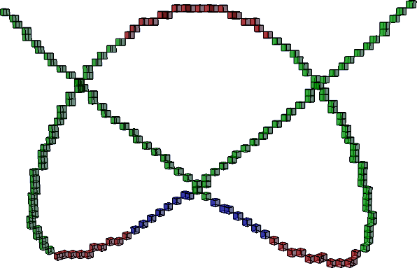
Knot $ 4_1 $ (see Knot_4_1.h)

Knot $ 4_3 $ (see Knot_4_3.h)

Knot $ 5_1 $ (see Knot_5_1.h)

Knot $ 5_2 $ (see Knot_5_2.h)

Knot $ 6_2 $ (see Knot_6_2.h)

Knot $ 7_4 $ (see Knot_7_4.h)

For more information about parametrized knots see https://www.maa.org/sites/default/files/images/upload_library/23/stemkoski/knots/page1.html by Lee Stemkoski of Adelphi University.

Geometric Transformations of 3D Parametric Curves

It is possible to rotate a 3D parametric curve around an arbitrary origin and an axis by using DecoratorParametricCurveTransformation.

Example below shows how to digitize an elliptic helix (see EllipticHelix.h) rotated by $ \frac{\pi}{3} $ around $ \omega = (\frac{1}{\sqrt{2}}, 0, \frac{1}{\sqrt{2}}) $.

Before using DecoratorParametricCurveTransformation, you must include the following headers:

#include "DGtal/geometry/curves/parametric/DecoratorParametricCurveTransformation.h"

#include "DGtal/images/RigidTransformation3D.h"

Then, you can construct the needed types as follows:

 typedef EllipticHelix < Space > MyHelix;
 typedef ForwardRigidTransformation3D < Space, RealPoint, RealPoint, Identity > ForwardTrans;
 typedef DecoratorParametricCurveTransformation < MyHelix, ForwardTrans > MyRotatedCurve;
 typedef NaiveParametricCurveDigitizer3D < MyRotatedCurve >  Digitizer;
 typedef typename NaiveParametricCurveDigitizer3D < MyRotatedCurve >::DigitalCurve MyDigitalCurve;

Also, we can state an instance of the curve i.e., elliptic helix of radii 30, 20 and distance between each period equal 1:

MyDigitalCurve digitalCurve;

MyHelix helix( 30, 20, 1 );

and we then state an instance of the decorator:

 double angle = M_PI/3.;
 RealVector axis ( 1., 0., 1. );
 ForwardTrans trans ( RealPoint ( 0, 0, 0 ), axis, angle, RealVector ( 0, 0, 0 ) );
 MyRotatedCurve rotCurve ( helix, trans );

Finally, we can compute a digitization together with the meta information by calling:

 Digitizer digitize;
 digitize.attach ( &rotCurve );
 digitize.init ( 0, MyHelix::getPeriod() * 10., 0.0001 );
 digitize.digitize( back_insert_iterator < MyDigitalCurve> ( digitalCurve ), back_insert_iterator < MyMetaData > ( metaData ) );

See exampleParamCurve3dDigitizationTransformationDecorator.cpp.

Handling Problems

In this section we discuss how to deal with problems such as curves that do not lead to a 26-connected digitization with the default parameters ( $ K_{NEXT}, t_{step} $).

Step values

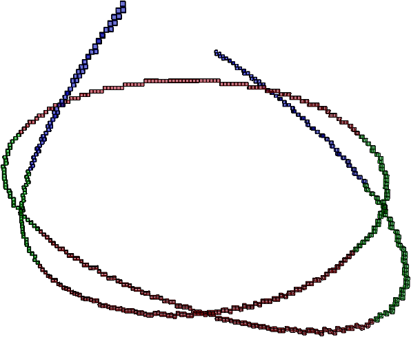
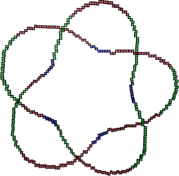
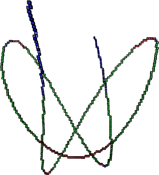
High step values can lead to disconnections in the digitization. For example, knot $3_1$ with scaling factors all equal 10 for a step 0.03 leads to

In order, to solve the above issue it is necessary to lower the step value e.g., to 0.003.

A high step value can also lead to wrong weights which can impact quality of the digitization.

Connectivity Problems

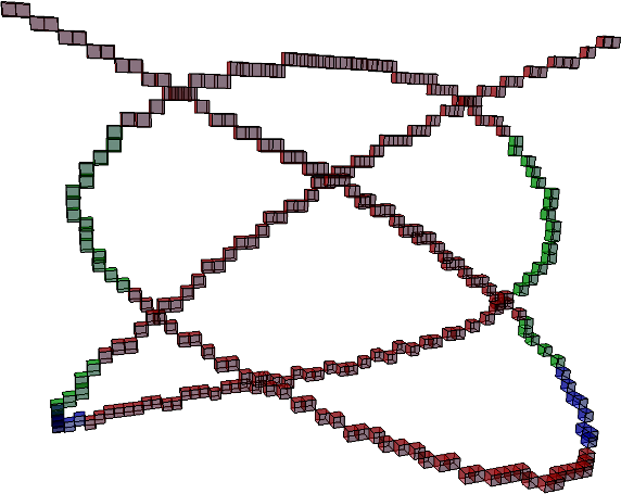
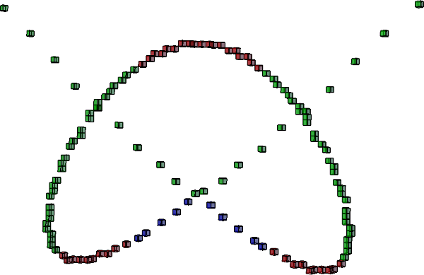
By trying to digitize a curve with a high, with respect to the grid, curvature we can arrive at a connectivity problems. For instance, if we consider an elliptic helix of radii 20, 1 and period distance 1, and $ K_{NEXT} = 2 $, we can observe connectivity issues i.e., there are at least three points such that they are 26-connected to each other and therefore the curve is not 26-connected in such a place.

In order to resolve the issue it is necessary to increase the value of $ K_{NEXT} $.

Table of Contents