computes a normal vector field over a digitized 3D implicit surface for several estimators.

Usage: ./estimators/generic3dNormalEstimators -p <polynomial> [options]

Computes a normal vector field over a digitized 3D implicit surface for several estimators (II|VCM|Trivial|True), specified with -e. You may add Kanungo noise with option -N. These estimators are compared with ground truth. You may then: 1) visualize the normals or the angle deviations with -V (if WITH_QGL_VIEWER is enabled), 2) outputs them as a list of cells/estimations with -n, 3) outputs them as a ImaGene file with -O, 4) outputs them as a NOFF file with -O, 5) computes estimation statistics with option -S.

Allowed options are :

-h,--help                             Print this help message and exit
-p,--polynomial TEXT REQUIRED         the implicit polynomial whose zero-level defines the shape of interest.
-N,--noise FLOAT=0                    the Kanungo noise level l=arg, with l^d the probability that a point at distance d is flipped inside/outside.
-a,--minAABB FLOAT=-10                the min value of the AABB bounding box (domain)
-A,--maxAABB FLOAT=10                 the max value of the AABB bounding box (domain)
-g,--gridstep FLOAT=1                 the gridstep that defines the digitization (often called h).
-e,--estimator TEXT:{True,VCM,II,Trivial}=True
                                      the chosen normal estimator: True | VCM | II | Trivial
-R,--R-radius FLOAT=5                 the constant for parameter R in R(h)=R h^alpha (VCM).
-r,--r-radius FLOAT=3                 the constant for parameter r in r(h)=r h^alpha (VCM,II,Trivial).
-k,--kernel TEXT=hat                  the function chi_r, either hat or ball.
--alpha FLOAT=0                       the parameter alpha in r(h)=r h^alpha (VCM).
-t,--trivial-radius FLOAT=3           the parameter t defining the radius for the Trivial estimator. Also used for reorienting the VCM.
-E,--embedding INT=0                  the surfel -> point embedding for VCM estimator: 0: Pointels, 1: InnerSpel, 2: OuterSpel.
-o,--output TEXT=output               the output basename. All generated files will have the form <arg>-*, for instance <arg>-angle-deviation-<gridstep>.txt, <arg>-normals-<gridstep>.txt, <arg>-cells-<gridstep>.txt, <arg>-noff-<gridstep>.off.
-S,--angle-deviation-stats            computes angle deviation error and outputs them in file <basename>-angle-deviation-<gridstep>.txt, as specified by -o <basename>.
-x,--export TEXT=None                 exports surfel normals which can be viewed with ImaGene tool 'viewSetOfSurfels' in file <basename>-cells-<gridstep>.txt, as specified by -o <basename>. Parameter <arg> is None|Normals|AngleDeviation. The color depends on the angle deviation in degree: 0 metallic blue, 5 light cyan, 10 light green, 15 light yellow, 20 yellow, 25 orange, 30 red, 35, dark red, 40- grey
-n,--normals                          outputs every surfel, its estimated normal, and the ground truth normal in file <basename>-normals-<gridstep>.txt, as specified by -o <basename>.
-O,--noff                             exports the digital surface with normals as NOFF file <basename>-noff-<gridstep>.off, as specified by -o <basename>..
-V,--view TEXT                        view the digital surface with normals.  Parameter <arg> is None|Normals|AngleDeviation. The color depends on the angle deviation in degree: 0 metallic blue, 5 light cyan, 10 light green, 15 light yellow, 20 yellow, 25 orange, 30 red, 35, dark red, 40- grey.

Example of implicit surface (specified by -p):

ellipse : 90-3*x^2-2*y^2-z^2
torus : -1*(x^2+y^2+z^2+6*6-2*2)^2+4*6*6*(x^2+y^2)
rcube : 6561-x^4-y^4-z^4
goursat : 8-0.03*x^4-0.03*y^4-0.03*z^4+2*x^2+2*y^2+2*z^2
distel : 10000-(x^2+y^2+z^2+1000*(x^2+y^2)*(x^2+z^2)*(y^2+z^2))
leopold : 100-(x^2*y^2*z^2+4*x^2+4*y^2+3*z^2)
diabolo : x^2-(y^2+z^2)^2
heart : -1*(x^2+2.25*y^2+z^2-1)^3+x^2*z^3+0.1125*y^2*z^3
crixxi : -0.9*(y^2+z^2-1)^2-(x^2+y^2-1)^3

Implemented estimators (specified by -e):

True : supposed to be the ground truth for computations. Of course, it is only approximations.
VCM : normal estimator by digital Voronoi Covariance Matrix. Radii parameters are given by -R, -r.
II : normal estimator by Integral Invariants. Radius parameter is given by -r.
Trivial : the normal obtained by average trivial surfel normals in a ball neighborhood. Radius parameter is given by -r.

Note

:

This is a normal direction evaluator more than a normal vector evaluator. Orientations of normals are deduced from ground truth. This is due to the fact that II and VCM only estimates normal directions.
This tool only analyses one surface component, and one that contains at least as many surfels as the width of the digital bounding box. This is required when analysing noisy data, where a lot of the small components are spurious. The drawback is that you cannot analyse the normals on a surface with several components.

Example:

Example of normal comparisons: You can estimate the normal vectors and compare the error with the true normals (option -V AngleDeviation):
# apply the Integral Invariant estimator (options -e II -r 8 ):

$ generic3dNormalEstimators -p "10000-(x^2+y^2+z^2+1000*(x^2+y^2)*(x^2+z^2)*(y^2+z^2))" -a -10 -A 10 -e II -r 8 -V AngleDeviation -g 0.05

# apply the Voronoi Covariance Measure based estimator (options -e VCM -r 8 ):

$ generic3dNormalEstimators -p "10000-(x^2+y^2+z^2+1000*(x^2+y^2)*(x^2+z^2)*(y^2+z^2))" -a -10 -A 10 -e VCM -R 20 -r 8 -V AngleDeviation -g 0.05

# to display source digital surface : visualize the normals and tape Key E to export surface (in exportedMesh.off)

$ generic3dNormalEstimators -p "10000-(x^2+y^2+z^2+1000*(x^2+y^2)*(x^2+z^2)*(y^2+z^2))" -a -10 -A 10 -e VCM -R 20 -r 8 -V Normals -g 0.05

# visualize generated file:

$ meshViewer -i exportedMesh.off

You should obtain such a result:

type visualization

digital surface

VCM angle-deviation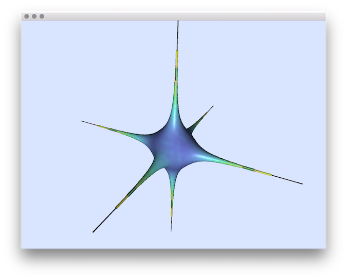

II angle-deviation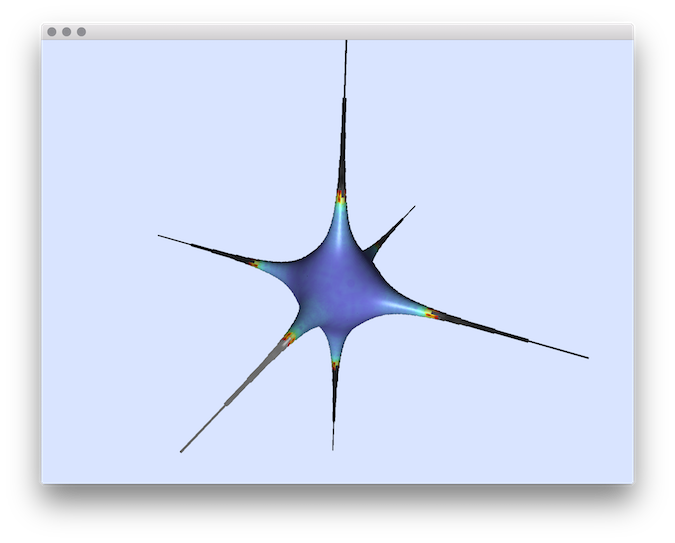
Example of normal visualization with noise add: This tool allows to add some noise on initial shape (option -N) and it is also possiblt to visualize the source shape by using the resulting normals:
# apply the Integral Invariant estimator (options -e II -r 6 ):

generic3dNormalEstimators -p "100-(x^2*y^2*z^2+4*x^2+4*y^2+3*z^2)" -a -10 -A 10 -e II -r 6 -V Normals -g 0.1 -N 0.3

# apply the Voronoi Covariance Measure based estimator (options -e VCM -r 8 ):

generic3dNormalEstimators -p "100-(x^2*y^2*z^2+4*x^2+4*y^2+3*z^2)" -a -10 -A 10 -e VCM -R 10 -r 5 -V Normals -g 0.1 -N 0.3

# apply the true normals:

./estimators/generic3dNormalEstimators -p "100-(x^2*y^2*z^2+4*x^2+4*y^2+3*z^2)" -a -10 -A 10 -e True -V Normals -g 0.1 -N 0.3

# to display source digital surface : tape Key E on previous displays to export surface (in exportedMesh.off)

# visualize generated file:

$ meshViewer -i exportedMesh.off

You should obtain such a result:

type	visualization
digital surface
VCM estimator
II estimator
True Normals

See also: generic3dNormalEstimators.cpp