Overview

The algorithm implemented in the class FrechetShortcut is the one presented in the article [110].
We present here the basic ideas of the algorithm and at the end, give pointers to the relative structures used in the implementation.

Given a polygonal curve, the curve simplification problem consists in computing another polygonal curve that (i) approximates the original curve, (ii) satisfies a given error criterion, (iii) with as few vertices as possible. This problem arises in a wide range of applications, such as geographic information systems (GIS), computer graphics or computer vision, where the management of the level of details is of crucial importance to save memory space or to speed-up analysis algorithms.

Given a 4- or 8-connected digital curve and a maximum error, we propose an algorithm that computes a simplification of the curve (a polygonal curve) such that the Fréchet distance between the original and the simplified curve is less than the error. The Fréchet distance is known to nicely measure the similarity between two curves. It can be intuitively defined considering a man walking his dog. Each protagonist walks along a path, and controls its speed independently, but cannot go backwards. The Fréchet distance between the two pathes is the minimal length of the leash required.

The algorithm implemented uses an approximation of the Fréchet distance, but a guarantee over the quality of the simplification is proved. Moreover, even if the theoretical complexity of the algorithm is in O(n log(n)), experiments show a linear behaviour in practice.

Fréchet distance

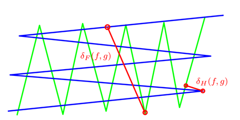
Given two curves $ f $ and $ g $ specified by functions $ f:[0,1] \rightarrow \mathbb{R}^2 $ and $g:[0,1] \rightarrow \mathbb{R}^2 $, and two non-decreasing continuous functions $ \alpha:[0,1] \rightarrow [0,1] $ and $ \beta:[0,1] \rightarrow [0,1] $ with $ \alpha(0)=0,\alpha(1)=1,\beta(0)=0,\beta(1)=1 $, the Fréchet distance $ \delta_F(f,g) $ between two curves f and g is defined as

$ \delta_F(f,g)=\inf_{\alpha,\beta} \max_{0\leq t \leq 1} d(f(\alpha(t)),g(\beta(t))) $

As illustrated in the figure below, contrary to the Hausdorff distance denoted by $ \delta_H(f,g) $, the Fréchet distance takes into account the course of the curves.

Difference between the Fréchet distance and the Hausdorff distance

Curve simplification problem

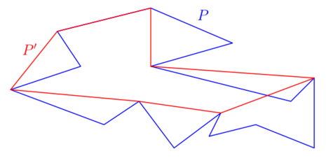
Given a polygonal curve $ P=\langle p_1,\dots p_n\rangle $, A curve $ P'=\langle p_{i_1},\dots p_{i_k}\rangle $ with $ 1=i_1 < \dots < i_k=n $ is said to simplify the curve $ P $. $ P(i,j) $ denotes the subpath from $ p_i $ to $ p_j $.

Given a pair of indices $ 1 \leq i \leq j \leq n $, $ \delta_F(p_ip_j,P) $ denotes the Fréchet distance between the segment $ p_ip_j $ and the part $ P(i,j) $ of the curve. For the sake of clarity, the simplified notation $ error(i,j) = \delta_F(p_ip_j,P) $ will sometimes be used. We also say that $ p_ip_j $ is a shortcut.

In other words, the vertices of $ P' $ form a subset of the vertices of $ P $, and the computation of $ P' $ comes down to the selection of "shortcuts" $ p_ip_j $.

The red curve P' is a simplification of the blue curve P

All in all, to find $ P' $ an $ \varepsilon $-simplification of $ P $ we have to:

Find shortcuts $ p_ip_j $ such that $ error(i,j) = \delta_F(p_ip_j,P) \leq \varepsilon $
Minimize the number of vertices of $ P' $.

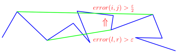
The following nice local property of the Fréchet distance proved in [3] will be very useful to prove a guarantee on the quality of the result produced by our algorithm (see illustration below):

Let $ P=\{p_1, p_2, \dots , p_n\} $ be a polygonal curve. \ For all $ i, j, l, r, 1 \leq i\leq l \leq r \leq j \leq n $, $ error(l,r) \leq 2 error(i,j) $.

In other words, the shortcuts of any $ \frac{\varepsilon}{2} $-simplification cannot strictly enclose the shortcuts of a $ \varepsilon $-simplification.

Illustration of the local property.

Guaranteed algorithm using an approximated distance

Definitions and overall algorithm

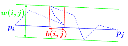
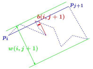
Using the exact Fréchet distance appears to be too expensive to design an efficient algorithm. Instead, we use an approximation of the Fréchet distance proposed in [1]. More precisely, they show that $error(i,j)$ can be upper and lower bounded by functions of two values namely $\omega(i,j)$ and $b(i,j)$. $\omega(i,j)$ is the width of the points of $P(i,j)$ in the direction $\overrightarrow{p_ip_j}$. $b(i,j)$ is the length of the longest backpath in the direction $\overrightarrow{p_ip_j}$.

Illustration of the definition of the width and the backpath length.

When a new point is considered, the width and backpath lengths may totally change.

We have the following property from [1] :

The Fréchet error of a shortcut $p_ip_j$ satisfies:

Using this Fréchet distance approximation to greedily compute a shortcut requires a fast update of the quantities $\omega(i,j)$ and $b(i,j)$ when a new point is taken into account. This is not an easy task since these values can change drastically as illustrated above.

Updating the width efficiently

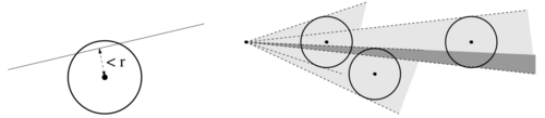
Instead of updating $\omega(i,j)$, it is enough to consider the maximal distance between any point of $P(i,j)$ and the vector $\overrightarrow{p_ip_j}$. This is done using the algorithm of Chan and Chin [20] illustrated below:

Given an origin point $p_i"$ and a set of points $P(i,j)$ we construct the set $S_{ij}$ of straight lines $l$ going through $p_i$ such that $\max_{p \in P(i,j)}d(p,l) \leq r$. As a result, deciding whether $d_{max}(i,j)$ is lower than $r$ or not is equivalent to checking whether the straight line $(p_i,p_j)$ belongs to $S_{ij}$ or not.

All in all, the update of the cone and the decision are both done in constant time.

The cone (dark gray) is computed incrementally as the intersection of the light gray cones.

Updating the backpath length efficiently

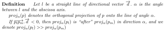
This update is trickier. When a new point $p_{j+1}$ is considered, we want to ckeck if there exists a backpath longer than a threshold in the direction $\overrightarrow{p_ip_j}$. Let us first give some definitions:

To do so, we consider a set of points named occulters* which are the furthest points for a given direction:

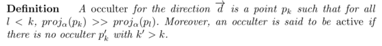
We can prove easily (see [110]) that the origin of the longest backpath is an occulter.

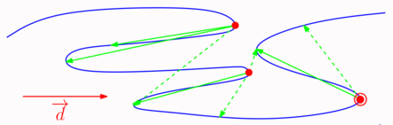
Occulters for the direction d in red. Green arrows represent backpathes: the length of the plain arrows is to be checked, whereas we know that the backpathes represented by dashed arrows are not the longest ones.

Considering whether the last movement $\overrightarrow{p_jp_{j+1}}$ is forward or backward in the direction $\overrightarrow{p_ip_j}$, we can decide if there is a new backpath possibly longer than the threshold or not. This is done according to Algorithm 2 below.

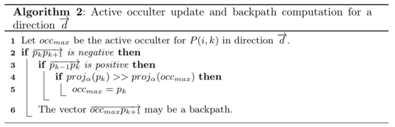
According to Algorithm 1 we see that Algorithm 2 must be applied for any possible direction for a given curve $P$, which is computationally expensive. However, the computation of backpathes can be mutualized in the case of digital curves. Indeed for a digital curve, the set of elementary shifts $\overrightarrow{p_jp_{j+1}}$ is well defined and it is actually possible to cluster the set of directions such that given an elementary shift $e$, this shift is either forward (positive) or backward (negative) for all the directions of the cluster.

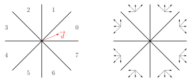
Left: The directions of the plane are clustered into 8 octants. For instance, direction

d is in octant 0. Right: Illustration of the positive (or forward) elementary shifts for each octant." @image latex clusters.png "Left: The directions of the plane are clustered into 8 octants. For instance, direction d is in octant 0. Right: Illustration of the positive (or forward) elementary shifts for each octant." If we now go back to Algorithm 2, we see that the result of the test lines 2-3 is the same for all the directions of a given octant. This test can thus be done jointly for all the directions of an octant. Nevertheless, to determine if a new point \_form#649 is the new active occulter (the furthest point for the direction studied), the projection of the current active occulter and the point \_form#649 on a direction are compared: the furthest of the two points is the active occulter. There, for any two points \_form#649 and \_form#650 the result of this comparison is not the same for all the directions of a given octant. This fact is illustrated in the figures below for the octant \_form#651: for any point \_form#650 in the grey area, and for any direction in octant \_form#651, \_form#650 is after \_form#271. for any point \_form#650 in the dashed area, and for any direction in octant \_form#651, \_form#271 is after \_form#650. in the white area, the order changes, as illustrated below. @image html zones.png "" @image latex zones.png "" @image html ordre_projections.png "For two points p and q and a direction α: on the left, q is after p, and is the active occulter for direction α, whereas on the right, p is after q and is the active occulter." @image latex ordre_projections.png "For two points p and q and a direction α: on the left, q is after p, and is the active occulter for direction α, whereas on the right, p is after q and is the active occulter." Algorithm 3 below puts together these observations to update the list of active occulters for one octant. @image html algo3.png "" @image latex algo3.png "" @subsection subsectDirections Memorizing the directions for which there exists a too long backpath From Algorithm 1, we see that the length of the longest backpath is tested for each new point, which defines a new direction. Moreover, we see from Algorithm 2 line 6 that for each negative shift, we can have as many backpathes as active occulters. All in all, testing individually all the possible backpathes when a new point is added is too expensive. To solve this problem, we propose to maintain a `‘set’' of the directions for which there exists a backpath of length greater than the error \_form#652. This set actually consists in a list of intervals: for a given backpath of length l and a given error \_form#652, the interval of directions for which the projection of the backpath is longer than \_form#652 is computed easily. The union of all these intervals is stored. @section sectQuality Quality of the result and complexity analysis @subsection subsectGuarantee A guaranteed algorithm An important issue when designing an algorithm that is known not to be optimal is to prove that the result of this algorithm is not so far from the optimal. In this work, the optimal solution is to compute the \_form#652-simplification of a digital curve P according to the Fréchet distance with a minimum number of vertices. The algorithm we propose here is not optimal for two reasons: it is greedy: the simplification is computed from a given starting point, in a given scanning order. the distance used is an approximation of the Fréchet distance. However, we prove that the number of vertices of the simplified curve computed by our algorithm is upper bounded by a function of the optimal solution: @image html lemma3.png "" @image latex lemma3.png ""

For more details about this proof, please refer to [110].

Complexity

The theoretical complexity of this algorithm is $\mathcal{O}(n\log(n_i))$, for a digital curve of $n$ points. $n_i$ is the number of intervals used to store the directions for which there exist a backpath of length greater than the error. $n_i$ is upper bounded by $n$. Nevertheless, experiments on noisy shapes show that the general behaviour of the algorithm in linear in time.

Implementation in DGtal

In DGtal, the FrechetShortcut should be used with a Curve object, using its PointsRange, as in the example below:

  Curve::PointsRange r = c.getPointsRange(); 
  
  typedef FrechetShortcut<Curve::PointsRange::ConstIterator,int> Shortcut;
  
  // Computation of one shortcut
  Shortcut s(error);
  
  s.init( r.begin() );
  while ( ( s.end() != r.end() )
          &&( s.extendFront() ) ) {}
  
 
 
  // Computation of a greedy segmentation
  
  typedef GreedySegmentation<Shortcut> Segmentation;
  
  Segmentation theSegmentation( r.begin(), r.end(), Shortcut(error) );
  
  // the segmentation is computed here
  Segmentation::SegmentComputerIterator it = theSegmentation.begin();
  Segmentation::SegmentComputerIterator itEnd = theSegmentation.end();
 
  for ( ; it != itEnd; ++it) {
    s=Shortcut(*it);
    trace.info() << s << std::endl;
    board << s; 
  }
  
  board.saveEPS("FrechetShortcutExample.eps", Board2D::BoundingBox, 5000 ); 
 

The function FrechetShortcut::extendFront() is called when a new point is added to the current shortcut. It calls FrechetShortcut::updateWidth() and FrechetShortcut::updateBackpath().

The function FrechetShortcut::updateWidth() implements the update of the width $\omega(i,j)$ and uses the subclass FrechetShortcut::Cone for the cone definition and manipulation.

The length of the longest backpath is managed in the function FrechetShortcut::updateBackpath(). It updates a vector of $8$ backpaths, one per each octant. The subclass FrechetShortcut::Backpath contains all the necessary structures

FrechetShortcut::Backpath::myQuad is the octant number
FrechetShortcut::Backpath::myOcculters is the list of occulters
FrechetShortcut::Backpath::addPositivePoint() is called when the next elementary move is forward for the octant
FrechetShortcut::Backpath::addNegativePoint() is called when the next elementary move is backward for the octant: it implements Algorithm 2 and calls updateOcculters()
FrechetShortcut::Backpath::updateOcculters() implements Algorithm 3
the list of interval used to memorize the directions for which there exist a too long backpath is implemented through FrechetShortcut::Backpath::myForbiddenIntervals using the Boost Interval Container Library (http://www.boost.org/doc/libs/1_52_0/libs/icl). It is updated with the function FrechetShortcut::Backpath::updateIntervals().

An output using the Board mecanism is provided (see example above to output an eps file).

Table of Contents