Geodesics In Heat using discrete polygonal calculus

Table of Contents

• The main algorithm
• The interface
• Examples

Author(s) of this documentation:

David Coeurjolly

Since

1.3

Part of package DEC package.

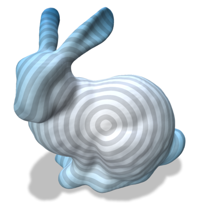
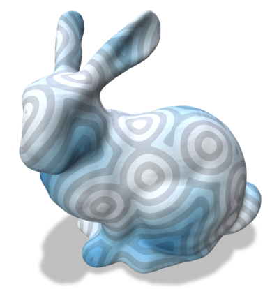
In this documentation page, we focus on an implementation of the "Geodesics In Heat method" ([39]). The main objective is to highlight the use of differential operators from Discrete differential calculus on polygonal surfaces to solve elementary PDEs.

Images are given by the dgtalCalculus-geodesic.cpp example file.

Warning

The implementation heavily relies on implicit operators with many Eigen based small matrix constructions, which has a huge overhead in Debug mode. Please consider to build the examples in Release (e.g. CMAKE_BUILD_TYPE variable) for high performance on large geometrical objects.

The main algorithm

The algorithm consists in three steps (see [39] for details):

• Given heat sources \( g \) at a mesh vertices, we first solve a heat diffusion problem: Integrate the heat flow \( u \) such that \(\Delta u = \frac{\partial u}{\partial t}\) using a single step backward Euler step: \((Id - t\Delta) u_t = g\)
• Evaluate the normalized field \( X = - \nabla u_t / \| \nabla u_t\|\)
• Solve the Poisson problem from the divergence of the normalized gradient field \(\Delta \phi = \nabla \cdot X\)

The computation involves discrete differential operator definitions (Laplace-Beltrami, gradient, divergence...) as well as linear solvers on sparse matrices. We do not go into the details of the discretization, please have a look to the paper if interested.

The interface

The class GeodesicsInHeat contains the implementation of the Geodesics in Heat method. It relies on the PolygonalCalculus class for the differential operators (Discrete differential calculus on polygonal surfaces).

First, we need to instantiate the GeodesicsInHeat class from an instance of PolygonalCalculus:

typedef PolygonalCalculus<SurfaceMesh<RealPoint,RealPoint>> Calculus;
Calculus aCalculus( mesh );
GeodesicsInHeat<Calculus> heat( aCalculus );

Then, we can prefactorized the solvers for a given a timestep \( dt\):

heat.init(dt);

Note

For a discussion on the timestep please refer to [39]. For short, the authors suggest a timestep in \( dt=m\cdot h^2\) for some constant \(m\) and \(h\) being the mean spacing between adjacent vertices.

Once prefactorized, we can add as many sources as we want using the method:

heat.addSource( aVertexIndex )
heat.addSource( anotherVertexIndex )
...

Note

the vertex index corresponds to the indexing system of the underlying SurfaceMesh instance.

The resulting geodesics diffusion is obtained by:

auto u = heat.compute();

Note

Once the init() has been called, you can iterate over addSource() and compute() for fast computations. If you want to change the timestep, you would need to call again the init() method.

Examples

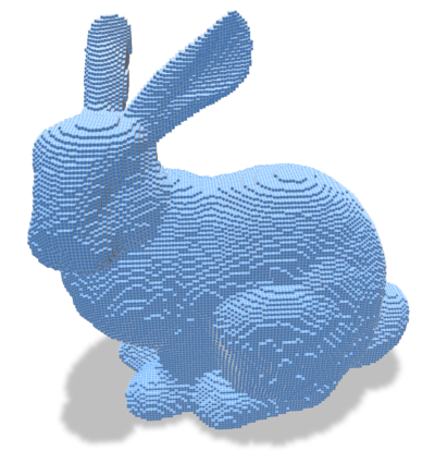
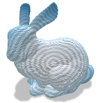
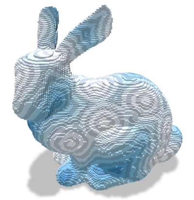
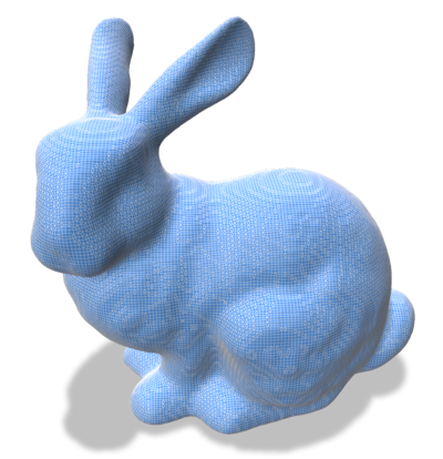
From dgtalCalculus-geodesic.cpp code on a digital surface and a regularization of the digital surface (see Digital surface regularization by normal vector alignment).

Input	Geodesics in heat	Geodesics with multiple (random) sources