
Table of Contents
- Date
- 2011/08/31
This part of the manual describes how to extract patterns from one-dimensional discrete structures (basically digital curves).
One-dimensional discrete structures
The goal is to provide tools that help in analysing any one-dimensional discrete structures in a generic framework. These structures are assumed to be constant, not mutable. This is a (not exhaustive) list of such structures used in digital geometry:
- digital curves
- 2d, 3d, nd
- 4-connected, 8-connected, disconnected
- interpixels, pixels
- open, closed
- chaincodes
Iterators/Circulators and Ranges.
Since these structures are one-dimensional and discrete, they can be viewed as a locally ordered set of elements, like a string of pearls. Two notions are thus important: the one of element and the one of local order, which means that all the elements (except maybe at the ends) have a previous and next element.
The concept of iterator is heavily used in our framework because it encompasses these two notions at the same time: like a pointer, it provides a way of moving along the structure (operator++, operator--) and provides a way of getting the elements (operator*).
In the following, iterators are assumed to be constant (because the structures are assumed to be constant) and to be at least bidirectionnal (ie. they are either bidirectionnal iterators or random access iterators). See Iterators and ranges.
GridCurve and FreemanChain.
Two objects are provided in DGtal to deal with digital curves: GridCurve and FreemanChain.
GridCurve describes, in a cellular space of dimension n, a closed or open sequence of signed d-cells (or d-scells), d being either equal to 1 or (n-1).
For instance, the topological boundary of a simply connected digital set is a closed sequence of 1-scells in 2d.
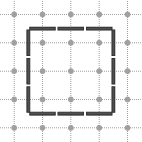
It stores a list of d-scells, but provides many ranges to iterate over different kinds of elements:
- SCellsRange to iterate over the d-scells
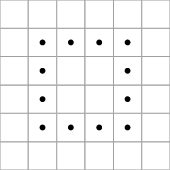
- PointsRange to iterate over the digital coordinates of the 0-scells that are directly incident to the d-scells
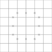
- MidPointsRange to iterate over the real coordinates of the d-scells
- ArrowsRange to iterate over the arrows coding the 1-scells. Note that an arrow is a pair point-vector: the point codes the digital coordinates of the 1-scell, the vector gives the topology and sign of the 1-scell.
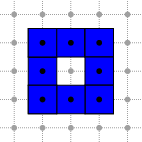
- InnerPointsRange to iterate over the digital coordinates of the n-scells that are directly incident to the (n-1)-scells.
- OuterPointsRange to iterate over the digital coordinates of the n-scells that are indirectly incident to the (n-1)-scells.
- IncidentPointsRange to iterate over the pairs of inner and outer points (defined as above)
- CodesRange to iterate over the codes {0,1,2,3} of the 1-scells (only available if n = 2)
You can get an access to these eight ranges through the following methods:
- getSCellsRange()
- getPointsRange()
- getMidPointsRange()
- getArrowsRange()
- getInnerPointsRange()
- getOuterPointsRange()
- getIncidentPointsRange()
- getCodesRange()
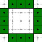
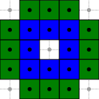
The different ranges for a grid curve whose chain code is 0001112223333 are depicted below.
FreemanChain is a 2-dimensional and 4-connected digital curve stored as a string of codes {0,1,2,3} as follows:
- 0 for a horizontal step to the right
- 1 for a vertical step to the up
- 2 for a horizontal step to the left
- 3 for a vertical step to the bottom
As GridCurve, it provides a CodesRange.
Each range has the following inner types:
- ConstIterator
- ConstReverseIterator
- ConstCirculator
- ConstReverseCirculator
And each range provides these (circular)iterator services:
- begin() : begin ConstIterator
- end() : end ConstIterator
- rbegin() : begin ConstReverseIterator
- rend() : end ConstReverseIterator
- c() : ConstCirculator
- rc() : ConstReverseCirculator
You can use these services to iterate over the elements of a given range as follows:
Since GridCurve and FreemanChain have both a method isClosed(), you can decide to use a classic iterator or a circulator at running time as follows:
Segments and on-line detection of segments.
In this section, we focus on parts of one-dimensional structures, called segment. More precisely, a segment is a valid and not empty range.
The concept concepts::CSegment refines boost::DefaultConstructible, boost::CopyConstructible, boost::Assignable, boost::EqualityComparable, and the one of constant range. It thus have the following inner types:
- ConstIterator : a model of bidirectional iterator
and the following methods:
- begin() : begin iterator
- end() : end iterator
Note that since a segment is a not empty range, we have the following invariant: begin() != end().
A class of segments \( \Sigma_P \) is a set of segments such that for each segment of the set, a given predicate P is true: \( \forall s \in \Sigma_P \), P(s) = true.
Segment computers are segments that can
- construct instances of their own type (or derived type)
- check whether a predicate (possibly not explicit) is true or not
CSegmentFactory is a refinement of CSegment and should define in addition the following nested types:
- Self (its own type)
- Reverse (like Self but based on reverse iterators)
Reverse is a type that behaves like Self but based on std::reverse_iterator<ConstIterator> instead of ConstIterator. Moreover, in order to build an instance of Self (resp. Reverse) from a segment computer, the following methods should be defined:
- Self getSelf() : returns an instance of Self
- Reverse getReverse() : returns an instance of Reverse
The returned objects may not be full copies of this, may not have the same internal state as this, but must be constructed from the same input parameters so that they can detect segments of the same class.
These methods are useful in segmentation algorithms when new segment computers must be created. An independant factory is not required since a segment computer is a factory for instances of its own type.
A segment computer is not a single concept, but actually several concepts that form a hierarchy. The five concepts that are used in segmentation algorithms are concepts::CIncrementalSegmentComputer, concepts::CForwardSegmentComputer, concepts::CBidirectionalSegmentComputer, concepts::CDynamicSegmentComputer and concepts::CDynamicBidirectionalSegmentComputer.
Incremental segment computers provides a way of incrementally detecting a segment belonging to a known class, ie. checking if P is true.
Note that the incremental constraint implies a constraint on P: for each iterator it from begin() to end(), P must be true for the range [begin(), it), so that a incremental segment computer can be initialized at a starting element and then can be extended forward to the neighbor elements while P remains true.
concepts::CIncrementalSegmentComputer is a refinement of concepts::CSegmentFactory and should provide in addition the following methods:
- void init ( const Iterator& it ) : set the segment to the element pointed to by it.
- bool extendFront () : return 'true' and extend the segment to the element pointed to by end() if it is possible, return 'false' and does not extend the segment otherwise.
- bool isExtendableFront () : return 'true' if the segment can be extended to the element pointed to by end() and 'false' otherwise (no extension is performed).
Detecting a segment in a range looks like this:
If the underlying structure is closed, infinite loops are avoided as follows:
Like any model of concepts::CIncrementalSegmentComputer, a model of concepts::CForwardSegmentComputer can control its own extension so that P remains true. However, contrary to models of concepts::CIncrementalSegmentComputer, it garantees that for each iterator it from begin() to end(), P must be true for the range [it, end()). This last constraint, together with the previous contraint on the range [begin(), it), implies that P is true for any subrange. This property is necessary to be able to incrementally check whether a segment is maximal (not included in a greater segment) or not.
As the name suggests, forward segment computers can only extend themselves in the forward direction, but this direction is relative to the direction of the underlying iterators (the direction given by operator++ for instances of Self, but the direction given by operator-- for instances of Reverse). They cannot extend themselves in two directions at the same time around an element contrary to bidirectional segment computers.
Any model of concepts::CBidirectionalSegmentComputer, which is a refinement of concepts::CForwardSegmentComputer, should define the following methods:
- bool extendBack () : return 'true' and extend the segment to the element pointed to by –begin() if it is possible, return 'false' and does not extend the segment otherwise.
- bool isExtendableBack () : return 'true' if the segment can be extended to the element pointed to by –begin() and 'false' otherwise (no extension is performed).
StabbingLineComputer and StabbingCircleComputer are both models of CBidirectionalSegmentComputer.
The concept concepts::CDynamicSegmentComputer is another refinement of concepts::CForwardSegmentComputer. Any model of this concept should define the following method:
- bool retractBack () : return 'true' and move the beginning of the segment to ++begin() if ++begin() != end(), return 'false' otherwise.
Finally, the concept concepts::CDynamicBidirectionalSegmentComputer is a refinement of both concepts::CBidirectionalSegmentComputer and concepts::CDynamicSegmentComputer and should define this extra method:
- bool retractFront () : return 'true' and move the end of the segment to –end() if begin() != –end(), return 'false' otherwise.
A model of concepts::CDynamicBidirectionalSegmentComputer is ArithmeticalDSSComputer, devoted to the dynamic recognition of DSSs, defined as a sequence of connected points \( (x,y) \) such that \( \mu \leq ax - by < \mu + \omega \) (see Debled and Reveilles, 1995).
Here is a short example of how to use this class in the 4-connected case:
This snippet is drawn from exampleArithmeticalDSSComputer.cpp. The resulting DSS is drawing below:
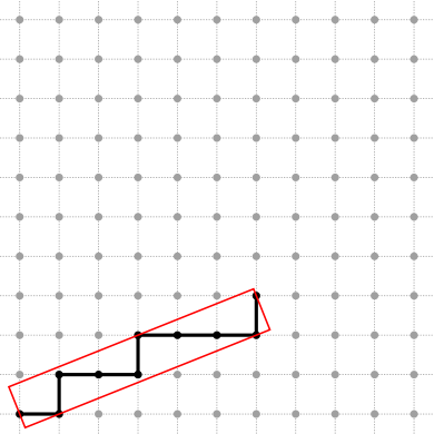
See Board2D: a stream mechanism for displaying 2D digital objects and Digital straight lines and segments
for the drawing mechanism.
As seen above, the code can be different if an iterator or a circulator is used as the nested ConstIterator type. Moreover, some tasks can be made faster for a given kind of segment computer than for another kind of segment computer. That's why many generic functions are provided in the file DGtal/geometry/curves/SegmentComputerUtils.h:
- maximalExtension, oppositeEndMaximalExtension, maximalSymmetricExtension,
- maximalRetraction, oppositeEndMaximalRetraction,
- longestSegment,
- firstMaximalSegment, lastMaximalSegment, mostCenteredMaximalSegment,
- previousMaximalSegment, nextMaximalSegment,
These functions are used in the segmentation algorithms introduced below.
Segments Extraction.
A given range contains a finite set of segments verifying a given predicate P.
A segmentation is a subset of the whole set of segments, such that:
i. each element of the range belongs to a segment of the subset and
ii. no segment contains another segment of the subset.
Due to (ii), the segments of a segmentation can be ordered without ambiguity (according to the position of their first element for instance).
Segmentation algorithms should verify the concept concepts::CSegmentation. A concepts::CSegmentation model should define the following nested type:
- SegmentComputerIterator: a model of the concept concepts::CSegmentComputerIterator
It should also define a constructor taking as input parameters:
- begin/end iterators of the range to be segmented.
- an instance of a model of concepts::CSegmentComputer.
Note that a model of concepts::CSegmentComputerIterator should define the following methods :
- default and copy constructors
- dereference operator: return an instance of a model of concepts::CSegmentComputer.
- intersectPrevious(), intersectNext(): return 'true' if the current segment intersects, respectively, the previous and the next one (when they exist), 'false' otherwise.
\subsection geometryGreedyDecomposition Greedy segmentation
The first and simplest segmentation is the greedy one: from a starting element, extend a segment while it is possible, get the last element of the resulting segment and iterate. This segmentation algorithm is implemented in the class GreedySegmentation.
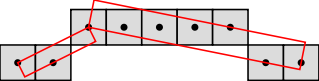
In the short example below, a digital curve stored in a STL vector is decomposed into 8-connected DSSs whose parameters are sent to the standard output.
If you want to get the DSSs segmentation of the digital curve when it is scanned in the reverse way, you can use the reverse iterator of the STL vector:
The resulting segmentations are shown in the figures below:
If you want to get the DSSs segmentation of a part of the digital curve (not the whole digital curve), you can give the range to process as a pair of iterators when calling the setSubRange() method as follow:
Obviously, [beginIt, endIt) has to be a valid range included in the wider range [curve.begin(), curve.end()).
Moreover, a part of a digital curve may be processed either as an independant (open) digital curve or as a part whose segmentation at the ends depends of the underlying digital curve. That's why 3 processing modes are available:
- "Truncate" (default), the extension of the last segment (and the segmentation) stops just before endIt.
- "Truncate+1", the last segment is extended to endIt too if it is possible, provided that endIt != curve.end().
- "DoNotTruncate", the last segment is extended as far as possible, provided that curve.end() is not reached.
In order to set a mode (before getting a SegmentComputerIterator), use the setMode() method as follow:
Note that the default mode will be used for any unknown modes.
The complexity of the greedy segmentation algorithm relies on the complexity of the extendFront() method of the segment computer. If it runs in (possibly amortized) constant time, then the complexity of the segmentation is linear in the length of the range.
Saturated segmentation.
A unique and richer segmentation, called saturated segmentation, is the whole set of maximal segments (a maximal segment is a segment that cannot be contained in a greater segment). This segmentation algorithm is implemented in the class SaturatedSegmentation.
In the previous segmentation code, instead of the line:
it is enough to write the following line:
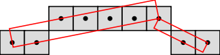
to get the following figure:
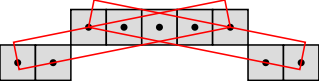
See convex-and-concave-parts.cpp for an example of how to use maximal DSSs to decompose a digital curve into convex and concave parts.
If you want to get the saturated segmentation of a part of the digital curve (not the whole digital curve), you can give the range to process as a pair of iterators when calling the setSubRange() method as follow:
Obviously, [beginIt, endIt) has to be a valid range included in the wider range [curve.begin(), curve.end()).
Moreover, the segmentation at the ends depends of the underlying digital curve. Among the whole set of
maximal segments that pass through the first (resp. last) element of the range, one maximal segment must be chosen as the first (resp. last) retrieved maximal segments. Several processing modes are therefore available:
- "First",
- "MostCentered" (default),
- "Last",
The mode i indicates that the segmentation begins with the i-th maximal segment passing through the first element and ends with the i maximal segment passing through the last element.
In order to set a mode (before getting a SegmentComputerIterator), use the setMode() method as follow:
Note that the default mode will be used for any unknown modes.
The complexity of the saturated segmentation algorithm relies on the complexity of the functions available for computing maximal segments (firstMaximalSegment, lastMaximalSegment, mostCenteredMaximalSegment, previousMaximalSegment and nextMaximalSegment), which are specialized according to the type of segment computer (forward, bidirectional and dynamic).
Let \( l \) be the length of the range and \( n \) the number of maximal segments. Let \( L_i \) be the length of the i-th maximal segments. During the segmentation, the current segment is extended:
- at most \( 2.\Sigma_{1 \leq i \leq n} L_i \) times in the forward case.
- exactly \( \Sigma_{1 \leq i \leq n} L_i \) times in the bidirectional case.
- \( l \) times in the dynamic case. (But in this case, the current segment is also retracted \( l \) times).
Moreover, note that \( \Sigma_{1 \leq i \leq n} L_i \) may be equal to \( O(l) \) (for instance for DSSs).