Table of Contents
Overview
The algorithm implemented in the class IntegralInvariantVolumeEstimator and IntegralInvariantCovarianceEstimator are detailed in the article [27] .
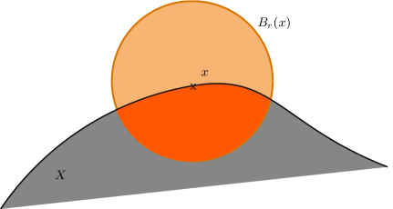
In geometry processing, interesting mathematical tools have been developed to design differential estimators on smooth surfaces based on Integral Invariant [94] [95] . The principle is simple: we move a convolution kernel along the shape surface and we compute integrals on the intersection between the shape and the convolution kernel, as follow in dimension 3:
\[ V_r(x) = \int_{B_r(x)} \chi(p)dp\ \]
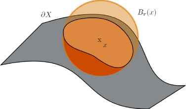
where \( B_r(x) \) is the Euclidean ball of radius \( r \), centered at \( x \) and \( \chi(p) \) the characteristic function of \( X \). In dimension 2, we simply denote \( A_r(x) \) such quantity (represented in orange color on the following figure).
Integral Invariant for curvature computation
In [26] , we have demonstrated that some digital integral quantities provide curvature information when the kernel size tends to zero for a sufficiently smooth shape. Indeed, at \( x \) of the surface \( X \) and with a fixed radius \( r \), we obtain convergent local curvature estimators \( \tilde{\kappa}_r(X,x) \) and \( \tilde{H}_r(X,x) \) of quantities \( \kappa(X,x) \) and \( H(X,x) \) respectively:
\[ \tilde{\kappa}_r(X,x) = \frac{3\pi}{2r} - \frac{3A_r(x)}{r^3},\quad \tilde{\kappa}_r(X,x) = \kappa(X,x)+ O(r) \]
\[ \tilde{H}_r(X,x) = \frac{8}{3r} - \frac{4V_r(x)}{\pi r^4},\quad \tilde{H}_r(X,x) = H(X,x) + O(r) \]
where \( \kappa_r(X,x) \) is the 2d curvature of \( X \) at \( x \) and \( H_r(X,x) \) is the 3d mean curvature of \( X \) at \( x \).
Then we showed that we can obtain local digital curvature estimators :
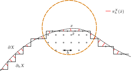
\[ \forall 0 < h < r,\quad \hat{\kappa}_r(Z,x,h) = \frac{3\pi}{2r} - \frac{3\widehat{Area}(B_{r/h}(\frac{1}{h} \cdot x ) \cap Z, h)}{r^3} \]
where \( \hat{\kappa}_r \) is an integral digital curvature estimator of a digital shape \( Z \subset ℤ^2 \) at point \( x \in \rm I\! R^2 \) and step \( h \). \( B_{r/h}(\frac{1}{h} \cdot x ) \cap Z, h) \) means the intersection between \( Z \) and a Ball \( B \) of radius \( r \) digitized by \( h \) centered in \( x \).
In the same way, we have in 3d :
\[ \forall 0 < h < r,\quad \hat{H}_r(Z',x,h) = \frac{8}{3r} - \frac{4\widehat{Vol}(B_{r/h}(\frac{1}{h} \cdot x ) \cap Z', h)}{\pi r^4}. \]
where \( \hat{H}_r \) is an integral digital mean curvature estimator of a digital shape \( Z' \subset ℤ^3 \) at point \( x \in \rm I\! R^3 \) and step \( h \) .
We have demonstrated in [26] that to prove the multigrid convergence with a convergence speed of \( O(h^{\frac{1}{3}}) \), the Euclidean radius of the kernel must follow the rule \( r = k_mh^{\alpha_m} \) ( \( \alpha_m = \frac{1}{3} \) provides better worst-case errors, so we will use this value).
Experimental results can be found at https://liris.cnrs.fr/jeremy.levallois/Papers/DGCI2013/ and https://liris.cnrs.fr/jeremy.levallois/Papers/AFIG2013/
Algorithm
Overall algorithm
The user part is rather simple by using only IntegralInvariantVolumeEstimator or IntegralInvariantCovarianceEstimator.
Since 2d curvature and 3d mean curvature are related to the volume between the shape and a ball centered on the border of the shape, we need to estimate this volume and use this value to get the curvature information. Then we parametrize our volume estimator IntegralInvariantVolumeEstimator by a functor to compute the curvature (in 2d: functors::IICurvatureFunctor and in 3d for the mean curvature: functors::IIMeanCurvature3DFunctor )
In 3d we can also compute the covariance matrix of the intersection between the shape and the ball centered on the border of the shape using IntegralInvariantCovarianceEstimator. This offers us the possibility to extract many differential quantities as: 3d Gaussian curvature, first and second principal curvatures, as well first and second principal curvature directions, normal vector or tangeant vector (functors::IIGaussianCurvature3DFunctor, etc. See file DGtal/geometry/surfaces/estimation/IIGeometricFunctors.h or namespace functors for the entire list).
Integral Invariant functors
All functors defined in IIGeometricFunctors.h have the same inititialization process: you need to use the default constructor, and initialize them with init() method. They will ask for a grid step ( \( h \)) and the Euclidean radius of the kernel ball ( \( r \)).
Integral Invariant estimators
As described below, this parameter \( r_e \) determines the level of feature detected by the estimator Since IntegralInvariantVolumeEstimator and (resp.) IntegralInvariantCovarianceEstimator are models of CSurfelLocalEstimator, they will follow rules inferred by it (init(), eval(), etc.). But some particular considerations are introduce. The following steps are the general usage of Integral Invariant estimators:
- First, you need to give them a functor on Volume (resp. Covariance matrix) on the constructor of the class (see above).
- You can also give them the cellular grid space model of CCellularGridSpaceND in which the shape is defined (Z3i::KSpace for example in 3d) and a point predicate model of concepts::CPointPredicate (the digital shape of interest, used to know if a point of the domain is inside or outside the shape), either in the constructor, or in the
attach()method.
- You can also give them the cellular grid space model of CCellularGridSpaceND in which the shape is defined (Z3i::KSpace for example in 3d) and a point predicate model of concepts::CPointPredicate (the digital shape of interest, used to know if a point of the domain is inside or outside the shape), either in the constructor, or in the
- Integral Invariant estimators need to know which size of ball you want to convolve around the shape boundary, so we need to call the
setParams(double)method with the digital radius of the ball ( \( \frac{r}{h} \)).- Warning
- II functors need the Euclidean radius of the ball, and II estimators the digital radius.
- Then, we can initialize our estimator, by calling
init()method. It requires the grid step of the shape \( h \), a begin and a end surfel iterator of the shape. This method will precompute all internal parameters for II estimator, as displacement masks optimization (see Technical details part below). - Finally, you can evaluate the estimator in two way:
- at a given (iterator of a) surface element (surfel) :
eval(it_surfel) - for a range of (iterators of) surface elements :
eval(it_begin, it_end, output). Hereoutputis an output iterator where results are given (std::back_insert_iterator for example).
- at a given (iterator of a) surface element (surfel) :
If you want to evaluate on a range of surfels, we recommend you to choose the second way. Indeed, some optimizations are available when the range of surfels is given with a 0-adjacency. Then, when you extract the digital surface of your shape, it's recommended to use a depth-first search (see DepthFirstVisitor for example). If none, no optimization are perform (it will be visible in performances for big shape).
Example code
It is important to consider a range of connected surfels when evaluating with Integral Invariant Curvature estimators in order to benefit the kernel optimization. Note that the methodology is the same with both IntegralInvariantVolumeEstimator and IntegralInvariantCovarianceEstimator. The only change is on the typedef of Functor/Estimator (see below):
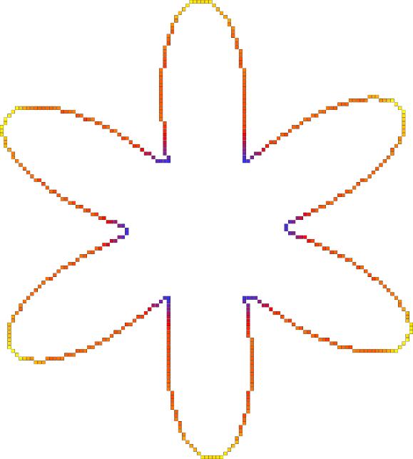
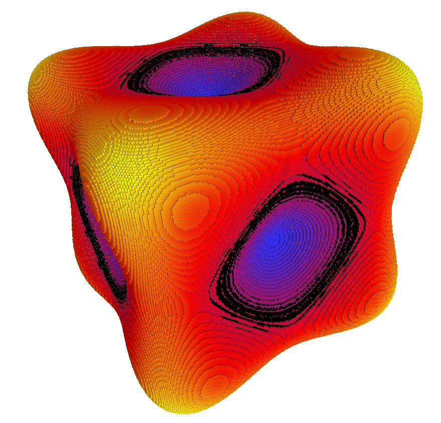
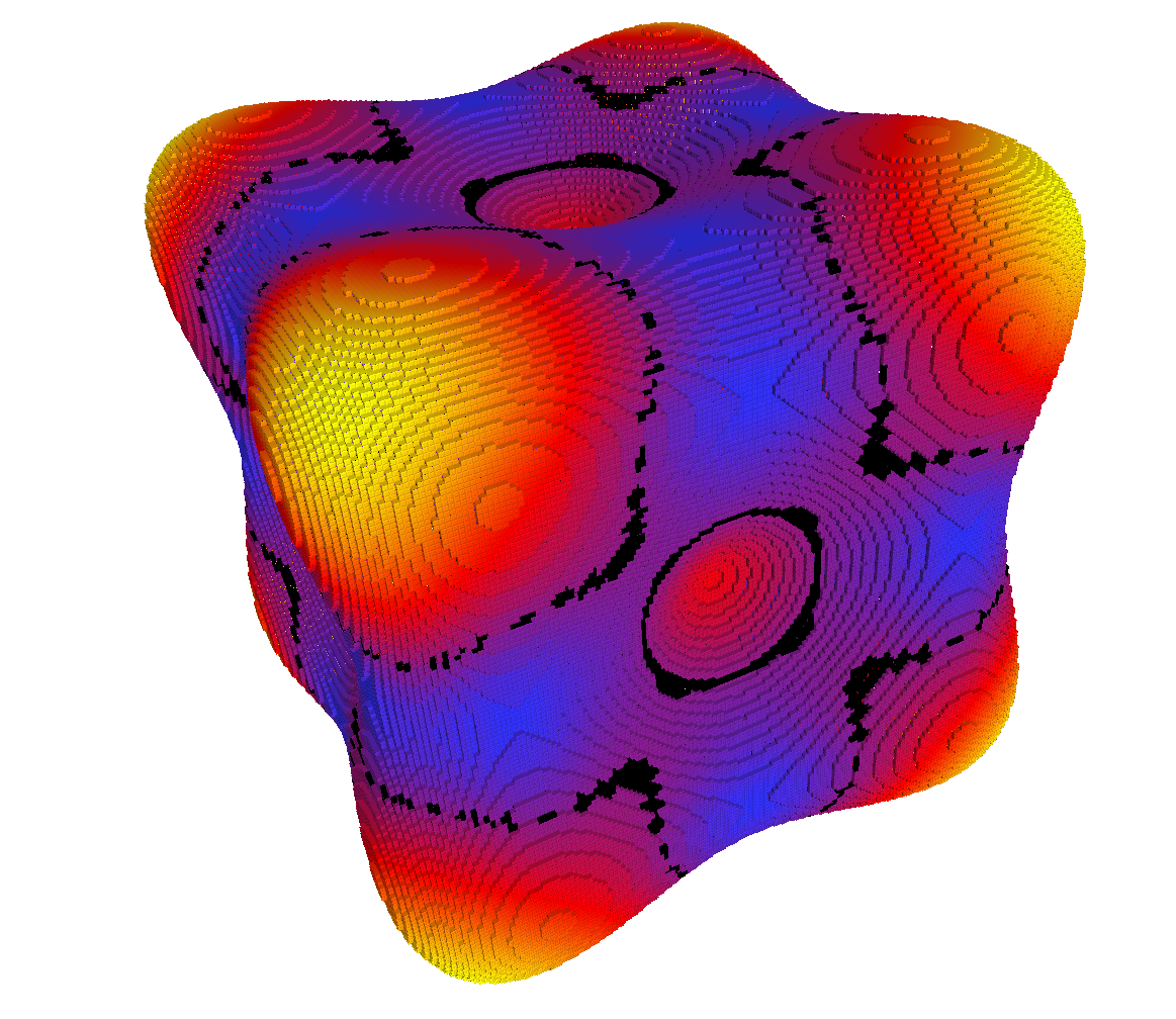
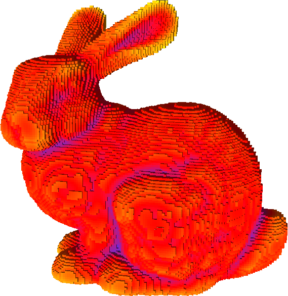
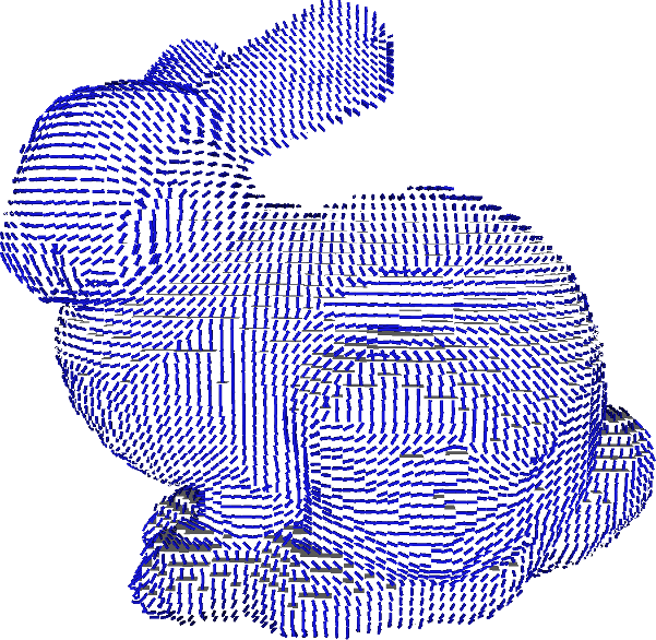
Some results
Here is some results in 2d and 3d :