3DCurvatureViewer

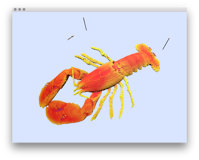
Computes and visualizes mean or gaussian curvature of binary shapes.

Vol file viewer, with curvature (mean or Gaussian, see parameters) information on surface. Blue color means lowest curvature Yellow color means highest curvature Red means the in-between

Uses IntegralInvariantCurvatureEstimation

See also

related article: Coeurjolly, D.; Lachaud, J.O; Levallois, J., (2013). Integral based Curvature Estimators in Digital Geometry. DGCI 2013. Retrieved from https://liris.cnrs.fr/publis/?id=5866

Usage: 3dCurvatureViewer -i file.vol –radius 5 –mode mean

Allowed options are:

-h [ --help ]                         display this message
-i [ --input ] arg                    .vol file
-r [ --radius ] arg                   Kernel radius for IntegralInvariant
-t [ --threshold ] arg (=8)           Min size of SCell boundary of an object
-l [ --minImageThreshold ] arg (=0)   set the minimal image threshold to
                                      define the image object (object defined
                                      by the voxel with intensity belonging
                                      to ]minImageThreshold,
                                      maxImageThreshold ] ).
-u [ --maxImageThreshold ] arg (=255) set the minimal image threshold to
                                      define the image object (object defined
                                      by the voxel with intensity belonging
                                      to ]minImageThreshold,
                                      maxImageThreshold] ).
-m [ --mode ] arg (=mean)             type of output : mean, gaussian, k1,
                                      k2, prindir1, prindir2 or normal
                                      (default mean)
-o [ --exportOBJ ] arg                Export the scene to specified OBJ/MTL
                                      filename (extensions added).
-d [ --exportDAT ] arg                Export resulting curvature (for mean,
                                      gaussian, k1 or k2 mode) in a simple
                                      data file each line representing a
                                      surfel.
--exportOnly                          Used to only export the result without
                                      the 3d Visualisation (usefull for
                                      scripts).
-s [ --imageScale ] arg               scaleX, scaleY, scaleZ: re sample the
                                      source image according with a grid of
                                      size 1.0/scale (usefull to compute
                                      curvature on image defined on
                                      anisotropic grid). Set by default to
                                      1.0 for the three axis.
-n [ --normalization ]                When exporting to OBJ, performs a
                                      normalization so that the geometry fits
                                      in [-1/2,1/2]^3

Below are the different available modes:

    - "mean" for the mean curvature
    - "gaussian" for the Gaussian curvature
    - "k1" for the first principal curvature
    - "k2" for the second principal curvature
    - "prindir1" for the first principal curvature direction
    - "prindir2" for the second principal curvature direction
    - "normal" for the normal vector

Example:

Now we compare the different curvature values from the two shapes:

3dCurvatureViewer -i $DGtal/examples/samples/lobster.vol -r 10 -l 40 -u 255 -m mean

You should obtain such a visualisation:

resulting visualisation of mean curvature.

See also

3dCurvatureViewer.cpp, 3DCurvatureViewerNoise