- Author(s) of this documentation:
- Jacques-Olivier Lachaud
Part of the Topology package.
This part of the manual describes how to define digital surfaces, closed or open. A lot of the ideas, concepts, algorithms, documentation and code is a backport from ImaGene [60]. Digital surfaces can be defined in very different way depending on input data, but they can be manipulated uniformly with class DigitalSurface, whichever is the dimension. Note that the topology within digital surfaces is computed on-the-fly. Since 0.9.4, one can precompute the topology of a 3D digital surface with class IndexedDigitalSurface. In some usages (typically local traversals), this can speed-up algorithms up to three times faster.
The following programs are related to this documentation: volToOFF.cpp, volMarchingCubes.cpp, volScanBoundary.cpp, volTrackBoundary.cpp, frontierAndBoundary.cpp, volBreadthFirstTraversal.cpp, trackImplicitPolynomialSurfaceToOFF.cpp, area-estimation-with-digital-surface.cpp, area-estimation-with-indexed-digital-surface.cpp
Introduction to digital surfaces
Possible definitions for digital surfaces
Although continuous surfaces are well defined as n-manifolds, a digital or discrete analog of surface is more tricky to define. Several methods have been explored to define consistent digital surfaces. We mention three approaches here.
- Surface as specific subsets of \( Z^n \), i.e. as sets of pixels in 2D, voxels in 3D, etc, with specific properties. This approach was proposed by Rosenfeld in the 70s. The set \( S \subset Z^n \) is a digital surface iff \( Z^n \setminus S \) is composed of two \( \alpha \)-connected components and if S is thin (i.e. if any point of S is removed, the preceding property does not hold). This approach is not too bad in 2D, becomes more complex in 3D (see the work of Morgenthaler and Rosenfeld or Malgouyres) and is unusable in practice. For instance the border of any digital object is generally not a surface.
- Surface as \( n-1 \)-dimensional cubical complexes. For example, if a digital object is a pure \( n \)-dimensional cubical complex, its boundary is naturally a \( n-1 \)-dimensional cubical complex. This seems at first sight a good approach, and it works well with well-composed pictures and images (see the work of Latecki et al.). The obtain complex is indeed a \( n-1 \)-manifold when realized in the Euclidean space. However, if the object contains any cross configuration (like two voxels connected by their edge, and the other two voxels adjacent to them are not in the object) then the preceding property does not hold anymore. Cubical complexes are thus interesting for representing objects, but not so interesting when one is interested by the geometry of its boundary.
- Surface as set of n-1-cells with some specific adjacencies. This approach is more or less the approach of Herman, Udupa and others, which was designed originally for tracking surfaces in a digital space. In 2D, this correspond to an interpixel approach. You choose first if you wish an interior adjacency (4-connectedness) or an exterior adjacency (8-adjacency). Two linels (or edges) are connected if they are point-connected and in case of a cross configuration they border the same interior (resp. exterior) pixel. The principle is the same in 3D, where a 2-cell (surfel) has edge-connected surfels with a preference in case of cross configuration.
We focus here on the last method to define digital surfaces.
Digital surface as a set of n-1-cells
Formally, the elements of the digital space \( Z^n \) are called spels, and often pixels in 2D and voxels in 3D. A surfel is a couple (u,v) of face-adjacent voxels. A digital surface is a set of surfels. It is obvious that a spel is a n-cell in the cellular grid decomposition of the space, while a surfel is clearly some oriented n-1-cell which is incident to the two n-cells u and v (see Cellular grid space and topology, unoriented and oriented cells, incidence).
Let s be some surfel. It is incident to two oriented voxels. By convention, its interior pixel is the one that is positively oriented.
We assume from now on that you have instantiated some cellular space K of type KSpace (see dgtal_ctopo_sec4), for instance with the following lines:
A surfel is an oriented \(n-1\)-cell, i.e. some SCell. Surfel may be obtained from spels by incidence relation. Reciprocally, you can use incidence to get spels.
The direct orientation to some cell s is the one that gives a positively oriented cell in the boundary or coboundary of s.
You may now for instance define the digital surface that lies in the boundary of some digital shape \( S \subset Z^n \) as the set of oriented surfels between spels of S and spels not in S. Algebraically, S is the formal of its positively oriented spels, and its boundary is obtained by applying the boundary operator on S.
Defining a digital surface as a set of surfels is not enough for geometry. Indeed we need to relate surfels together so as to have a topology on the digital surface. The first step is to transform the digital surface into a graph.
- Note
- From a properly oriented \(n-1\)-cell (i.e. a surfel), one can retreive the coordinates in \(Z^n\) of the associated interior / exterior grid points (voxel in 3d) using the KhalimskySpaceND::interiorVoxel and KhalimskySpaceND::exteriorVoxel methods.
Digital surface as a graph: adding adjacencies between surfels
The idea here is to connect surfels that share some \(n-2\)-cells. The obtained adjacency relations are called bel adjacencies in the terminology of Herman, Udupa and others. Generally an \(n-2\)-cell is shared by at most two \(n-1\)-cells, except in "cross configuration", symbolized below:
   O | X    X: interior spels               O a X
   - + -    O: exterior spels               b + c
   X | O    - and |: surfels a,b,c,d        X d O
            +: n-2-cell
A bel adjacency makes a deterministic choice to connect b to d and a to c when interior, and b to a and c to d when exterior. This choice has to be made along each possible pair of directions when going nD. In DGtal, this is encoded with the class SurfelAdjacency.

The following snippet shows the interior surfel adjacency (i.e. (6,18)-surfaces).
Once the adjacency has been chosen, it is possible to determine what are the adjacent surfels to a given surfel. More precisely, any surfel (or \(n-1\)-cell) has exactly \(2n-2\) adjacent surfels (for closed surfaces). More precisely, it has exactly 2 adjacent surfels along directions different from the orthogonal direction of the surfel.
In fact, we can be even more precise. We can use orientation to orient the adjacencies consistently. Given two surfels sharing an \(n-2\)-cell, this cell is positively oriented in the boundary of one surfel and negatively oriented in the boundary of the other. We have thus that there are \(n-1\) adjacent cells in the direct orientation (positive) and \(n-1\) adjacent cells in the indirect orientation (negative). The direct adjacent surfels look like:
The class SurfelNeighborhood is the base class for computing adjacent surfels. You may use it as follow, but generally this class is hidden for you since you will have more high-level classes to move on surfaces.
Generally, methods SurfelNeighborhood::getAdjacentOnSpelSet, SurfelNeighborhood::getAdjacentOnDigitalSet, SurfelNeighborhood::getAdjacentOnPointPredicate, SurfelNeighborhood::getAdjacentOnSurfelPredicate are used to find adjacent surfels.
Since we have defined adjacencies between surfels on a digital surface, the digital surface forms a graph (at least in theory).
Tracking digital surfaces
This section shows how to extract the boundary of a digital set, given some predicate telling whether we are inside or outside the surface.
Constructing digital surfaces by scanning
Given a domain and a predicate telling whether we are inside or outside the object of interest, it is easy to determine the set of surfels by a simple scanning of the space. This is done for you by static methods Surfaces::uMakeBoundary and Surfaces::sMakeBoundary.
The following snippet shows how to get a set of surfels that is the boundary of some predicate on point by a simple scan of the whole domain (see volScanBoundary.cpp).
Constructing digital surfaces by tracking
In many circumstances, it is better to use the above mentioned graph structure of digital surfaces. For instance it may be used to find the surface just by searching it by adjacencies. This process is called tracking. This is done for you by static method Surfaces::trackBoundary.
The following snippet shows how to get a set of surfels that is the boundary of some predicate on point given only a starting surfel and by tracking (see volTrackBoundary.cpp).
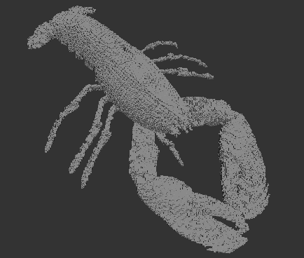
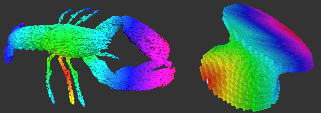
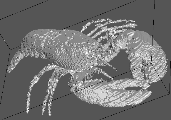
On the lobser.vol volume, volScanBoundary.cpp extracts 155068 surfels in 3866ms, while volTrackBoundary.cpp extracts 148364 surfels in 351ms.
# Commands
$ ./examples/topology/volScanBoundary ../examples/samples/lobster.vol 50 255
$ ./examples/topology/volTrackBoundary ../examples/samples/lobster.vol 50 255
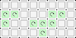
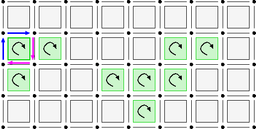
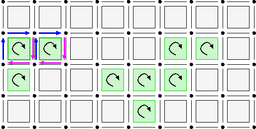
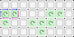
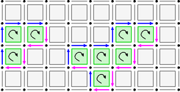
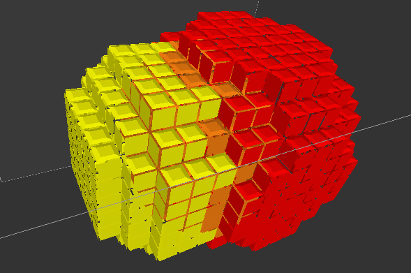
In the case you know beforehands that your surface is closed (i.e. without boundary), you should use preferentially Surfaces::trackClosedBoundary. This technique only follows direct adjacent surfels and extracts the whole surface when it is closed. This process can be illustrated as follows:
Other constructions by tracking: 2D contours, surface connected components, 2D slices in 3D surface
You can have a look at page Helpers for digital surfaces to see how to construct directly a 2D contour in \( Z^2 \), how to get the set of surface components, how to get 2D contours as slices onto a 3D surface.
You may also use the template class DigitalSurface2DSlice, which, given a tracker on a digital surface, computes and store a 2d slice on the associated surface. You may after visit the slice with iterators or circulators.
- See also
- digitalSurfaceSlice.cpp
High-level classes for digital surfaces
Digital surfaces arise in many different contexts:
- an explicit set of oriented surfels
- the boundary of an explicit set of spels
- the boundary of an explicit set of digital points
- the boundary of a set of digital points, defined implicitly by a predicate: Point -> bool
- a set of oriented surfels, defined implicitly by a predicate: Surfel -> bool
- a set of oriented surfels, implicitly by a predicate: Oriented Surfel -> bool
- the boundary of a region in a labelled image
- the frontier between two regions in a labelled image
- ...
Since there are so many digital surfaces, it is necessary to provide a mechanism to handle them generically. The class DigitalSurface will be the common proxy to hide models of concepts::CDigitalSurfaceContainer.
A common architecture for digital surfaces
Since there may be several types of digital surfaces, there are several container classes for them. All of them follow the concept concepts::CDigitalSurfaceContainer. Essentially, a model of this class should provide methods begin() and end() to visit all the surfels, and a Tracker which allows to move by adjacencies on the surface. A Tracker should be a model of concepts::CDigitalSurfaceTracker. The architecture is sumed up below:
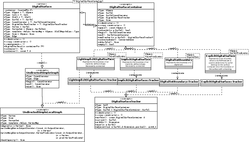
Models of digital surface containers
For now, the implemented digital surface container are (realization of concepts::CDigitalSurfaceContainer):
- model DigitalSetBoundary, parameterized by a cellular space and a digital set. Represents the boundary of a digital set (a set of digital points, considered as the set of pixels/voxels/spels of the space).
- model ImplicitDigitalSurface, parameterized by a cellular space and a predicate Point->bool. Represents the (connected) boundary of shape defined implicitly by a predicate. Computes at instanciation the set of surfels by a tracking algorithm.
- model LightImplicitDigitalSurface, parameterized by a cellular space and a predicate Point->bool. Represents the (connected) boundary of shape defined implicitly by a predicate. Do not compute at instanciation the set of surfels, but rather visits the surface on demand.
- model SetOfSurfels, parameterized by a cellular space and a set storing surfels. Represents an arbitrary set of surfels stored explicitly.
- model ExplicitDigitalSurface, parameterized by a cellular space and a predicate Surfel->bool. Represents a (connected) set of surfels defined implicitly by a predicate. Computes at instanciation the set of surfels by a tracking algorithm.
- model LightExplicitDigitalSurface, parameterized by a cellular space and a predicate Surfel->bool. Represents a (connected) set of surfels defined implicitly by a predicate. Do not compute at instanciation the set of surfels, but rather visits the surface on demand.
Depending of what is your digital surface, you should choose your container accordingly:
- an explicit set of oriented surfels: model SetOfSurfels, or if you wish to keep only one connected component, the model ExplicitDigitalSurface together with a model of concepts::CSurfelPredicate on your set.
- the boundary of an explicit set of spels: either convert it to a DigitalSet and use model DigitalSetBoundary, or use model ImplicitDigitalSurface and a concepts::CPointPredicate on your set of spels (require connectedness).
- the boundary of an explicit set of digital points: model DigitalSetBoundary directly
- the boundary of a set of digital points, defined implicitly by a predicate Point -> bool: model ImplicitDigitalSurface and a start surfel
- a set of oriented surfels, defined implicitly by a predicate Surfel -> bool: model ExplicitDigitalSurface and a start surfel.
- the boundary of a region in a labelled image: model ExplicitDigitalSurface and a start surfel, and the class functors::BoundaryPredicate, which is model of concepts::CSurfelPredicate.
- the frontier between two regions in a labelled image: model ExplicitDigitalSurface and a start surfel, and the class functors::FrontierPredicate, which is model of concepts::CSurfelPredicate.
Light versions of containers should be preferred in mostly two cases:
- The digital surface is big and you do not wish to keep it in memory. This is probably the case when tracking some implicit function and outputing it in some stream.
- The digital surface is likely to evolve (i.e. the predicate do not give the same response at a point/surfel depending on when it is called).
Relating a digital surface to some container
The following snippet shows how to create a digital surface associated to a LightImplicitDigitalSurface. The LightImplicitDigitalSurface is connected to a shape described by a predicate on point (a simple digital set). The full code is in volBreadthFirstTraversal.cpp.
Once this is done, the object digSurf is a proxy to your container. Here the dynamically allocated object is acquired by the digital surface, which will take care of its deletion.
- Note
- This creation of the container and the connection to a digital surface takes almost no time, since the chosen container (Light...) is lazy: the whole surface has not been extracted yet.
A digital surface is a graph, example of breadth-first traversal
Any DigitalSurface is a model of concepts::CUndirectedSimpleGraph (a refinement of concepts::CUndirectedSimpleLocalGraph). Essentially, you have methods DigitalSurface::begin() and DigitalSurface::end() to visit all the vertices, and for each vertex, you obtain its neighbors with DigitalSurface::writeNeighbors. You may thus for instance use the class BreadthFirstVisitor to do a breadth-first traversal of the digital surface.
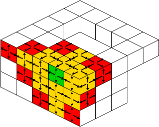
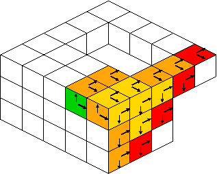
We may extract the whole surface by doing a breadth-first traversal on the graph. The snippet below shows how to do it on any kind of digital surface, whatever the container.
Here, we only use it to get the maximal distance to the starting bel. A second pass could be done to display cells with a color that depends on the distance to the starting surfel.
We may call it as follows
# Commands
$ ./examples/topology/volBreadthFirstTraversal ../examples/samples/lobster.vol 50 255
$ ./examples/topology/volBreadthFirstTraversal ../examples/samples/Al.100.vol 0 1
$ ./examples/topology/volBreadthFirstTraversal ../examples/samples/cat10.vol 1 255
to get these pictures:
- Note
- In fact, the specific container LightImplicitDigitalSurface performs itself a breadth-first traversal to extract its vertices by itself. Therefere, you may use a simple begin() and end() to get the vertices in this order, when your container is a LightImplicitDigitalSurface.
Boundary and frontiers examples of digital surface
Surfels of a digital surface can also be defined by a predicate telling whether or not some surfel belongs to it. Given an image of labels, the class functors::BoundaryPredicate and functors::FrontierPredicate are such predicates:
- functors::BoundaryPredicate ( KSpace, Image, l ) is a predicate returning true for a surfel s iff the interior spel of s has label
lwhile the exterior spel of s has label different froml. - functors::FrontierPredicate ( KSpace, Image, l1, l2 ) is a predicate returning true for a surfel s iff the interior spel of s has label
l1while the exterior spel of s has labell2.
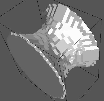
Using container ExplicitDigitalSurface, we can very simply define digital surfaces that are connected boundary of frontiers in some image. The following snippet is an excerpt from frontierAndBoundary.cpp.
Running it give the pictures:
The digital surface graph is a combinatorial manifold
Umbrellas and faces
We have shown before that a digital surface has a dual structure that is the graph whose vertices are n-1-cells and whose arcs are (almost) n-2-cells. We can go further and use n-3-cells to define faces on this graph. This is related to the concept of umbrellas in 3D (see [93]). More precisely, given a start surfel, an incident n-2-cell (the separator) and an incident n-3-cell (the pivot), one can turn around the pivot progressively to get a face. This gives precisely in 3D the dual to a digital surface that is a kind of marching-cube surface (see [65], [66]).
The main class for computing umbrellas is the class UmbrellaComputer. Turning around the pivot means moving the face and the separator once (in the track direction), such that the pivot is the same (ie +p), the track and separator directions being updated. Repeating this process a sufficient number of times brings the umbrella back in its original position, except in the case when the DigitalSurface has a boundary touching the pivot. You may use it to compute umbrellas given a tracker on your surface.
You may look at file testUmbrellaComputer.cpp to see how to use this class directly.
Vertices, arcs and faces on a digital surface
However, it is simpler to use directly the methods defined in DigitalSurface. It offers three types: DigitalSurface::Vertex, DigitalSurface::Arc, DigitalSurface::Face to get the combinatorial structure of the surface. An arc is an oriented edge, a face is a sequence of edges that is closed when the pivot is not on the boundary and open otherwise.
The following code lists the faces of a DigitalSurface object, and for each face it lists the coordinates of its vertices.
DigitalSurface provides you with many methods to get faces from edges or vertices and reciprocally.
- DigitalSurface::outArcs (Vertex): the range of outgoing arcs from the given vertex.
- DigitalSurface::inArcs (Vertex): the range of ingoing arcs from the given vertex.
- DigitalSurface::facesAroundVertex (Vertex): the range of faces containing this vertex [v]: 0 in 2D, 4 in 3D, 12 in 4D, 2(n-1)(n-2) in nD. Since DGtal 1.0, in 3D, the 4 faces may be ordered counterclockwise around the vertex (seen from the exterior), if the user specifies it.
- DigitalSurface::head (Arc): the head vertex of the given arc
- DigitalSurface::tail (Arc): the tail vertex of the given arc
- DigitalSurface::opposite (Arc): the opposite arc of the given arc (may not exist if the arc lies on some boundary).
- DigitalSurface::arc (Vertex,Vertex): the arc from the first vertex toward the second.
- DigitalSurface::facesAroundArc (Arc): the range of faces incident to a given arc. Empty in 2D. 1 face in 3D, 2 in 4D and so one, n-2 in nD. Returned faces may be open.
- DigitalSurface::verticesAroundFace (Face): the sequence of vertices that touches this face. The order follows the order of incident arcs.
- DigitalSurface::allFaces (): the set of all faces of the digital surface (open and closed faces).
- DigitalSurface::allClosedFaces (): the set of all closed faces of the digital surface.
- DigitalSurface::allOpenFaces (): the set of all open faces of the digital surface.
- DigitalSurface::computeFace ( UmbrellaComputer::State ): compute the face from a given umbrella state.
- DigitalSurface::separator ( Arc ): the separator of a given arc (the n-2-cell between the two surfels forming the arc).
- DigitalSurface::pivot ( Face ): the positively oriented n-3-cell that is the pivot of the face.
Application to export surface in OFF format
In 3D, you may use faces to transform an arbitrary digital surface into a polygonal manifold (closed or open). You can for instance directly the method DigitalSurface::exportSurfaceAs3DOFF to do so, or look at its code to see how it works.
The following snippets of file volToOFF.cpp show how to extract all surfels in an image and then how to export the surface in OFF format. The output is a surface that is very much the classical marching-cube surface, except that vertices lies in the middle of the edge.
Precomputed 3D digital surface with IndexedDigitalSurface
Digital surfaces are built upon digital surface containers. Although containers may be very differnt, digital surfaces provide a uniform interface to visit them and to explore their topology. But they are merely just an interface. Hence neighbors, umbrellas, and sometimes even vertices are recomputed on-the-fly as needed.
In some cases, it is a better idea to compute the topology once and for all and to store it as fixed arrays. This is the purpose of class IndexedDigitalSurface.
- Note
- For now, the class IndexedDigitalSurface can only handle 3D digital surface containers. It is because the topology is stored in a half-edge data structure (HalfEdgeDataStructure), which can only represents 2D combinatorial manifolds.
Creating an IndexedDigitalSurface
Similarly to a DigitalSurface, one creates an IndexedDigitalSurface with a model of digital surface container (concepts::CDigitalSurfaceContainer). The following snippet creates it from a DigitalSetBoundary (the boundary of a ball of radius 3 here).
- Note
- We recall that, as for a DigitalSurface, an IndexedDigitalSurface represents the topology of the dual of the cubical cell complex formed by the surfels and their incident cells. Hence vertices are surfels, edges correspond to linels (more precisely a couple of surfels sharing an edge) and faces correspond to pointels (more precisely an umbrella of surfels around this pointels). It is because the topology of the primal digital surface seen as a 2-dimensional cubical complex is not a 2-manifold in general. However, for its dual, we are able to define a 2-manifold.
Guide for using an IndexedDigitalSurface
Once the indexed surface is created, you may use it as a DigitalSurface. First it is a model of graph (concepts::CUndirectedSimpleGraph). Hence traversal operations and visitors apply. The main difference is that vertices, arcs and faces are now numbered consecutively starting from 0. Therefore you have methods to get a surfel from its vertex index, a linel from its arc index, a pointel from its face index.
- IndexedDigitalSurface::surfel : gets the surfel associated with a given vertex index.
- IndexedDigitalSurface::linel : gets the linel associated with a given arc index.
- IndexedDigitalSurface::pointel : gets the pointel associated with a given face index.
- IndexedDigitalSurface::surfels : gets the whole mapping vertex index -> surfel.
- IndexedDigitalSurface::linels : gets the whole mapping arc index -> surfel.
- IndexedDigitalSurface::pointels: gets the whole mapping face index -> surfel.
- IndexedDigitalSurface::getVertex: gets the vertex index of the given (oriented) surfel.
- IndexedDigitalSurface::getArc: gets the arc index of the given (oriented) linel (i.e. its separator).
- IndexedDigitalSurface::getFace: gets a face index of the given pointel (i.e. its pivot). Note that several faces may have the same pivot (up to four).
An indexed digital surface associates positions to its vertices (see IndexedDigitalSurface::position and IndexedDigitalSurface::positions).
Then, most the services of DigitalSurface described in The digital surface graph is a combinatorial manifold are available in IndexedDigitalSurface.
- IndexedDigitalSurface::outArcs (Vertex): the vector of outgoing arcs from the given vertex.
- IndexedDigitalSurface::inArcs (Vertex): the vector of ingoing arcs from the given vertex.
- IndexedDigitalSurface::facesAroundVertex (Vertex): the vector of faces containing this vertex [v]: 4 faces in 3D.
- IndexedDigitalSurface::head (Arc): the head vertex of the given arc
- IndexedDigitalSurface::tail (Arc): the tail vertex of the given arc
- IndexedDigitalSurface::opposite (Arc): the opposite arc of the given arc (may not exist if the arc lies on some boundary).
- IndexedDigitalSurface::arc (Vertex,Vertex): the arc from the first vertex toward the second.
- IndexedDigitalSurface::facesAroundArc (Arc): the vector of faces incident to a given arc. Only 1 face in 3D. Returned face may be open.
- IndexedDigitalSurface::verticesAroundFace (Face): the sequence of vertices that touches this face. The order follows the order of incident arcs.
- IndexedDigitalSurface::allFaces (): the vector of all faces of the digital surface, i.e. an array containing 0, 1, 2, ..., nbFaces()-1.
The following services are also provided:
- IndexedDigitalSurface::allArcs (): the vector of all arcs of the digital surface, i.e. an array containing 0, 1, 2, ..., nbArcs()-1.
- IndexedDigitalSurface::allVertices (): the vector of all vertices of the digital surface, i.e. an array containing 0, 1, 2, ..., nbVertices()-1.
- IndexedDigitalSurface::allBoundaryArcs (): the vector of all arcs of the digital surface lying on its boundary.
- IndexedDigitalSurface::allBoundaryVertices (): the vector of all vertices of the digital surface lying on its boundary.
- IndexedDigitalSurface::next (Arc): the next arc along the (only) incident face.
- IndexedDigitalSurface::faceAroundArc (Arc): the (only) face incident to a given arc (in 3D). Returned face may be open.
- IndexedDigitalSurface::isVertexBoundary (Vertex): true iff it lies on the boundary.
- IndexedDigitalSurface::isArcBoundary (Arc): true iff it lies on the boundary.
When using an IndexedDigitalSurface instead of a DigitalSurface ?
You should use an IndexedDigitalSurface when:
- the digital surface is never modified
- you use a lot traversal operations (like computing k-neighborhoods everywhere)
- you use a lot surface operations (order of faces around a vertex)
- you do not use too much the cell geometry and topology but just their combinatorial relations
- or you need to number your cells consecutively.
You should use a DigitalSurface when
- you use a lot the geometry and topology of cells
- the digital surface is sometimes modified (then use light containers)
- you just iterate over surfels and perform few neighborhood operations.
Examples area-estimation-with-digital-surface.cpp and area-estimation-with-indexed-digital-surface.cpp illustrate the similarities of classes DigitalSurface and IndexedDigitalSurface as well as their slight differences. They show how to estimate the area of a digital sphere.