The following programs are related to this documentation: geometry/volumes/fullConvexityAnalysis3D.cpp , geometry/volumes/fullConvexityThinning3D.cpp , geometry/volumes/fullConvexityLUT2D.cpp , geometry/volumes/fullConvexityCollapsiblePoints2D.cpp , geometry/volumes/fullConvexityShortestPaths3D.cpp , geometry/volumes/fullConvexitySphereGeodesics.cpp .

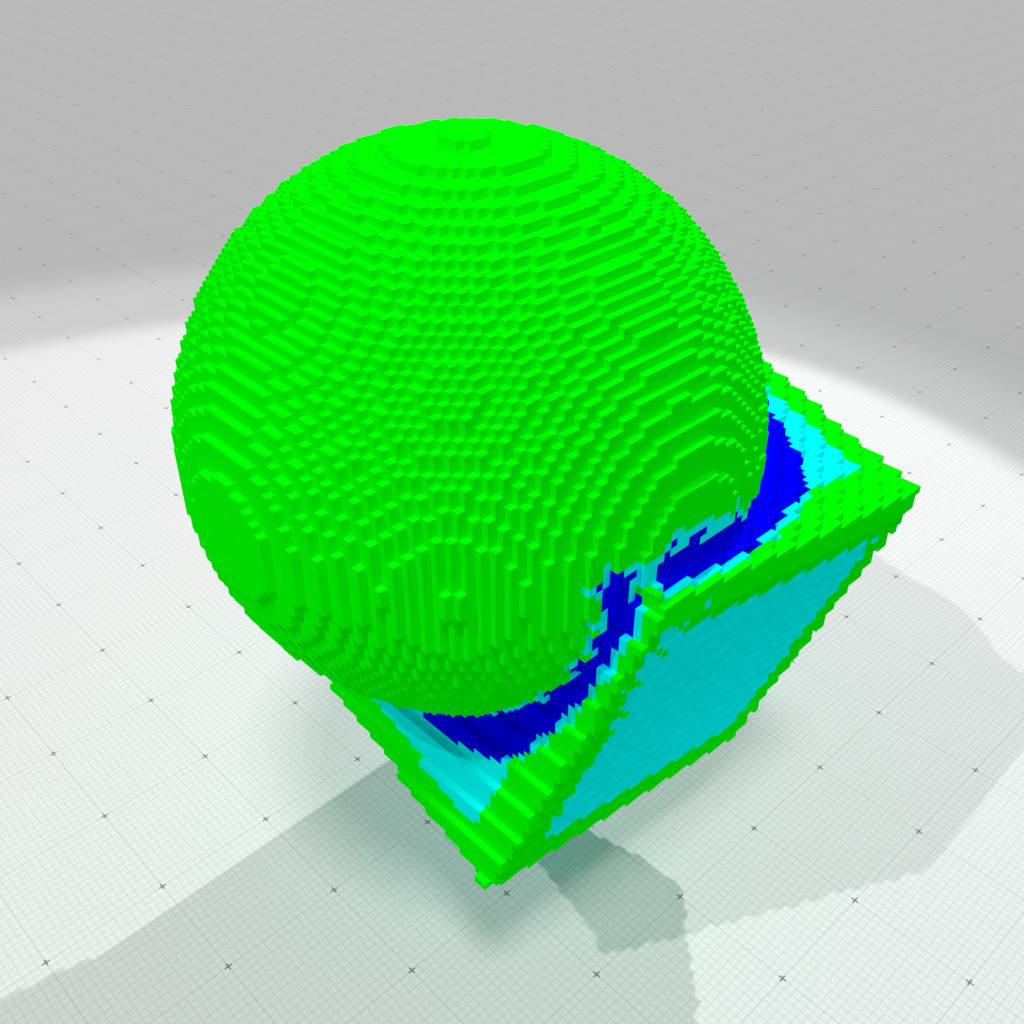
Local convexity analysis

Full convexity is stable by intersection with an half-space with axis-aligned normal vector and integer intercept. Hence if \( X \) is fully convex, and \( N_k(x) \) is a \( (2k+1)^d \) neighborhood around point x, then \( X \cap N_k(x) \) is also fully convex.

This shows that a fully convex set is locally fully convex everywhere. Reciprocally local analysis with full convexity gives information on the local geometry:

\( X \) is k-convex at x, whenever \( X \cap N_k(x) \) is fully convex;
\( X \) is k-concave at x, whenever \( (\mathbb{Z}^d \setminus X) \cap N_k(x) \) is fully convex;
\( X \) is k-planar at x, whenever it is both k-convex and k-concave at x;
otherwise \( X \) is k-atypical at x.

Due to the stability properties of full convexity, one may observe that \( k+1 \)-convexity at x implies \( k \)-convexity at x, the same holds for concavity and planarity. Taking the contraposition indicates that \( k \)-atypicality implies \( k+1 \)-atypicality.

Class NeighborhoodConvexityAnalyzer offers many services to check these properties in an efficient way. It stores look-up tables to perform these services efficiently in 2D for 3x3 neighborhood, and also uses memoization to speed-up computations (useful in dimension greater than 2 and/or when the neighborhood is larger).

The following snippet shows how you can use it.

#include "DGtal/geometry/volumes/NeighborhoodConvexityAnalyzer.h"
...
using namespace Z3i;
auto params = SH3::defaultParameters();
auto bimage = SH3::makeBinaryImage( "Al.100.vol", params );
auto K      = SH3::getKSpace( bimage );
 
// Set up a memoizer of up to 50000 configurations.
NeighborhoodConvexityAnalyzer< KSpace, 1 > NCA( K, 50000 );
 
// Compute all immediate interior points (inner boundary).
auto surface = SH3::makeDigitalSurface( bimage, K, params );
std::vector< Point > points;
for ( auto s : (*surface) )
  {
    Dimension k = K.sOrthDir( s );
    auto voxel  = K.sIncident( s, k, K.sDirect( s, k ) );
    Point p     = K.sCoords( voxel );
    points.push_back( p );
  }
// Analyse inner boundary points
for ( auto x : points )
  {
    nca.setCenter( x, *bimage );                         // center neighborhood on point x
    bool  cvx = nca.isFullyConvex( true );               // check 1-convexity
    bool ccvx = nca.isComplementaryFullyConvex( false ); // check 1-concavity
    ...
  }

You may have a look at geometricAnalysis3D.cpp to have a more complete example.

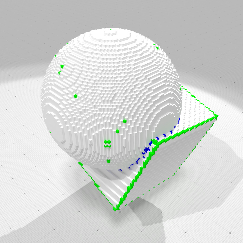
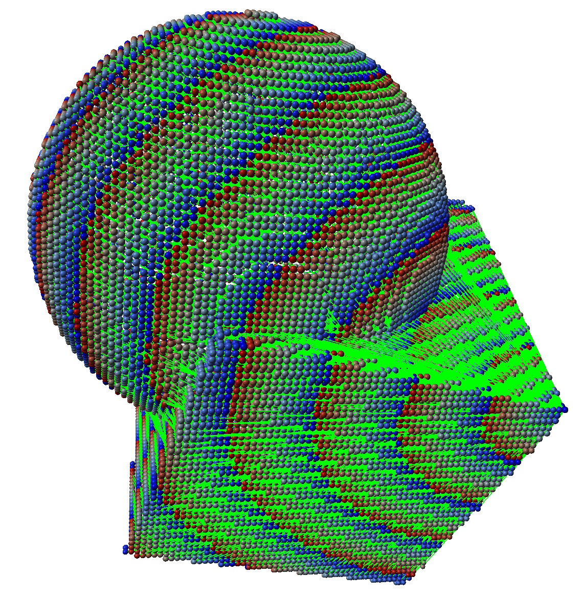
Full convexity analysis at scale 1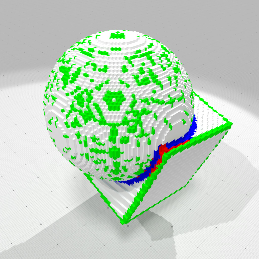

Full convexity analysis at scale 2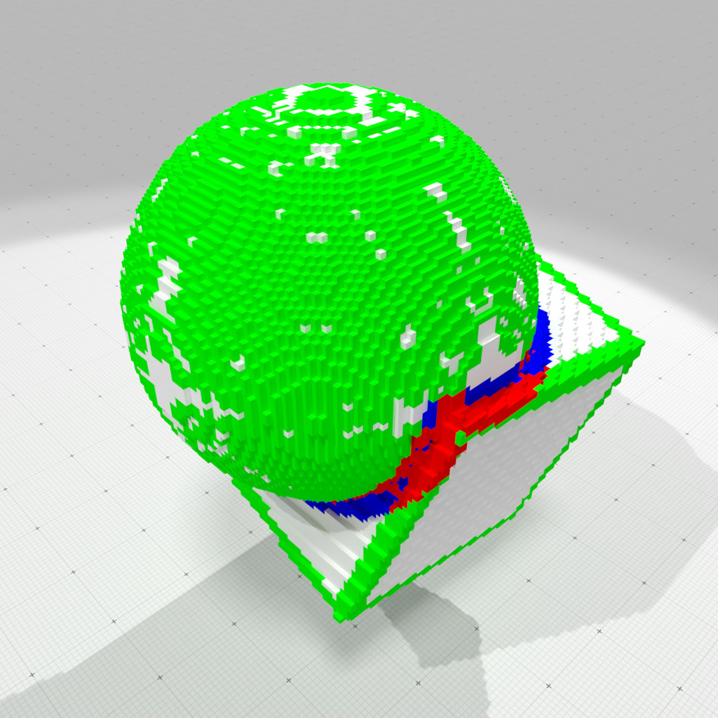

Full convexity analysis at scale 3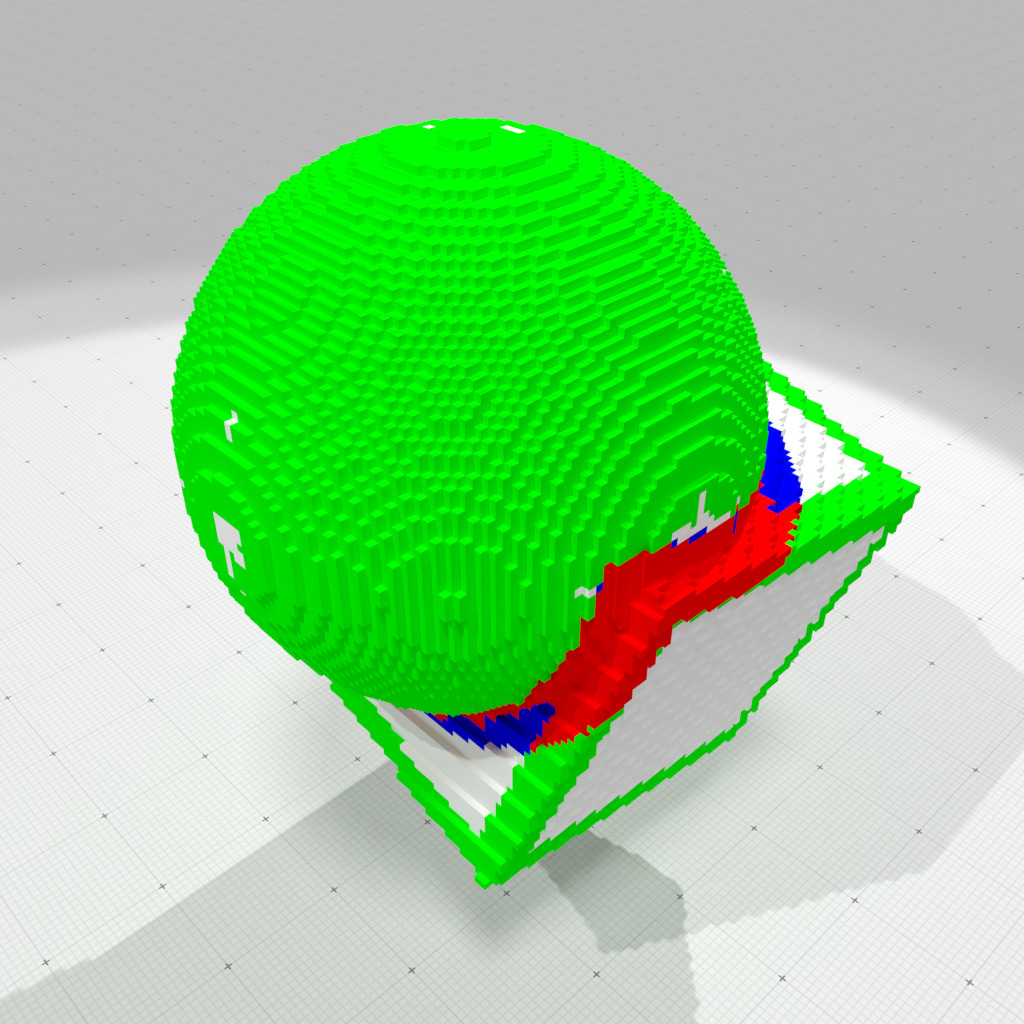

Full convexity analysis at scale 4

Full convexity multiscale analysis (scales 1-5)

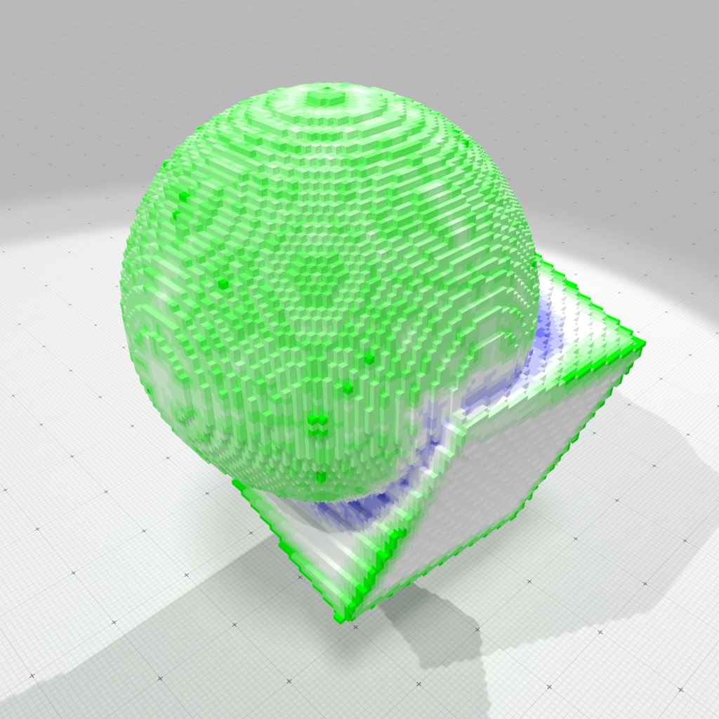
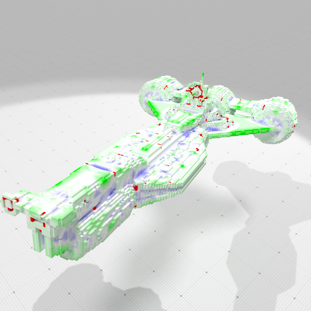
Full convexity smooth multiscale analysis (scales 1-5)

Tangency and shortest paths

Definition of tangency and shortest paths

Tangency or subconvexity is a derived concept from full convexity. Let \( X \subset \mathbb{Z}^d \) some arbitrary digital set. Then the digital set \( A \subset \mathbb{Z}^d \) is said to be digitally k- subconvex to \( X \) whenever \( C^d_k \lbrack \mathrm{Conv}(A) \rbrack \subset C^d_k \lbrack X \rbrack \). And \( A \) is said to be fully (digitally) subconvex to \( X \) whenever it is digitally k- subconvex to \( X \) for \( 0 \le k \le d \).

We also say that \( A \) is tangent to \( X \). The elements of \( A \) are said to be cotangent (in \( X \)). Note that necessarily \( A \subset X \).

A path \( \gamma \) from a to b in \( X \) is then a sequence a points \( \gamma=(x_i)_{i=0,\ldots,n} \), such that \( x_0 = a \), \( x_n = b \), and for all \( i \in \{ 0, \ldots, n-1 \} \), it holds that \( \{ x_i, x_{i+1} \} \) is tangent to \( X \).

We can embed in the Euclidean space the path \( \gamma \) simply by joining its consecutive points by Euclidean straight line segments. Its length is then just the Euclidean length of its embedding.

The cotangency relations define a graph on \( X \), which can be weighted by the length of the Euclidean segments joining cotangent points. Shortest paths on this graph are of course path in the above mentioned sense.

Implementation with TangencyComputer class

The class TangencyComputer offers some services to check tangency and to compute shortest paths:

TangencyComputer::TangencyComputer requires a cellular grid space big enough to include the future digital object
TangencyComputer::init defines the points of the digital object
several accessors are provided to get the space, the points (which are indexed in the same order as initialization), their indices and the cell cover
TangencyComputer::arePointsCotangent checks if two points are cotangent
TangencyComputer::getCotangentPoints returns all the indices of the cotangent points to a given point
TangencyComputer::shortestPath builds the shortest path between a source and a destination
TangencyComputer::shortestPaths builds all shortest paths to a given source, or builds shortest paths between sources and a set of possible destinations
TangencyComputer::makeShortestPaths returns a ShortestPaths object, which allows you to compute shortest paths efficiently

To use it, you should include the following headers

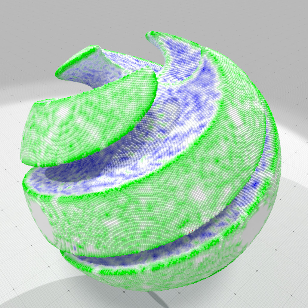
#include "DGtal/geometry/volumes/TangencyComputer.h"

Shortest paths to a source

We use here a TangencyComputer::ShortestPaths object to compute and store all shortest paths to a given target point.

  TangencyComputer< KSpace > TC( K );
  TC.init( points.cbegin(), points.cend() );
  auto SP = TC.makeShortestPaths( opt );
  SP.init( start0 ); //< set source
  double last_distance = 0.0;
  while ( ! SP.finished() )
    {
      last_distance = std::get<2>( SP.current() );
      SP.expand();
    }
  std::cout << "Max distance is " << last_distance << std::endl;

The object stores for each point:

its ancestor in the breadth first traversal (following the sequence of ancestors gives you the shortest path to the target(s))
its distance to the (closest) target.

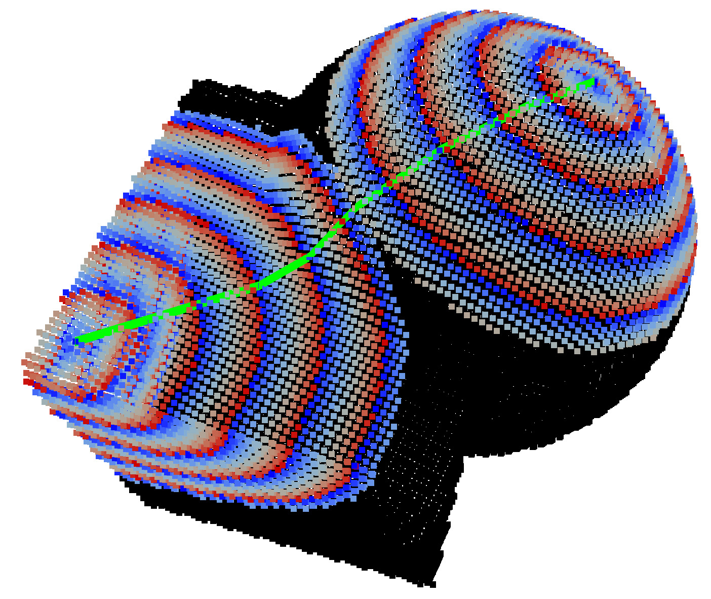
Example fullConvexityShortestPaths3D.cpp illustrates that kind of computations, giving the distance of each object point to the specified target.

Geodesic distances and geodesics on cube+sphere shape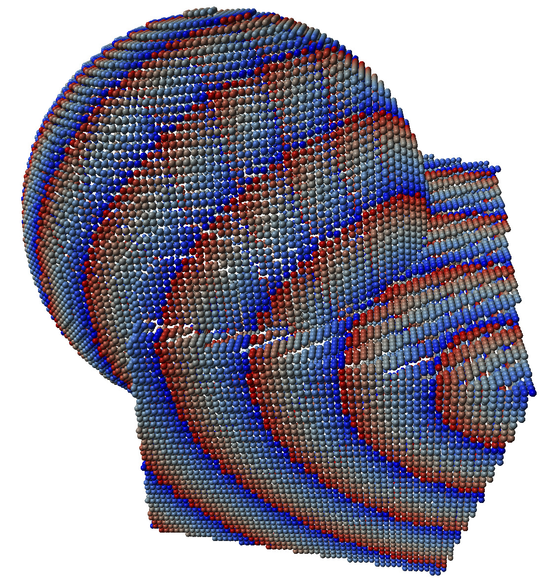

Geodesic distances on cube+sphere shape

You may obtain nicer views by exporting your result to an OBJ format and then render it.

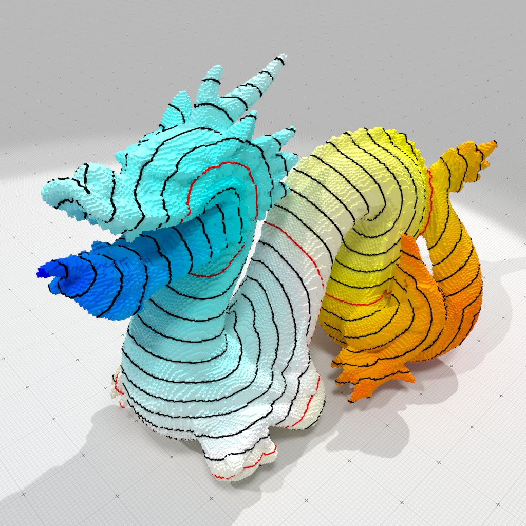
Geodesic distances on dragon digital surface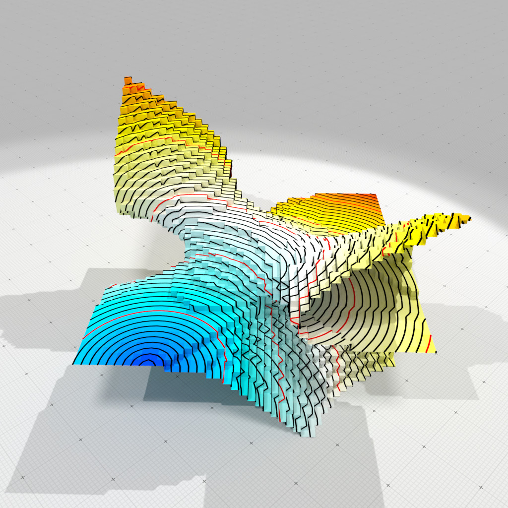

Geodesic distances on butterfly digital surface

Shortest path between a source and a target

If you wish to compute only one path, generally it is faster to use breadth first traversal from both the source and the target and stop at first collision. This is already implemented in TangencyComputer::shortestPath, using two TangencyComputer::ShortestPaths objects. The snippet below shows you how it is computed internally:

  auto SP0 = TC.makeShortestPaths( opt );
  auto SP1 = TC.makeShortestPaths( opt );
  SP0.init( start0 );     //< source point
  SP1.init( start1 );     //< target point
  std::vector< Index > Q; //< the output shortest path
  while ( ! SP0.finished() && ! SP1.finished() )
    {
      auto n0 = SP0.current();
      auto n1 = SP1.current();
      auto p0 = std::get<0>( n0 );
      auto p1 = std::get<0>( n1 );
      SP0.expand();
      SP1.expand();
      if ( SP0.isVisited( p1 ) )
        {
          auto c0 = SP0.pathToSource( p1 );
          auto c1 = SP1.pathToSource( p1 );
          std::copy(c0.rbegin(), c0.rend(), std::back_inserter(Q));
          Q.pop_back();
          std::copy(c1.begin(), c1.end(), std::back_inserter(Q)); 
          break;
        }
    }
  // Q is empty if there is no path.

Shortest path between two points

Approximated shortest paths to speed-up computation

Classes TangencyComputer and TangencyComputer::ShortestPaths offer a way to considerably speed up shortest paths computation if one tolerates a little bit of approximation. Several methods accept a distance parameter K. If K is greater than \( \sqrt{d} \), then shortest paths are exact (meaning all extracted paths are the shortest possible in the sense of the above mentioned algorithm), but if you give a lower value (from \( \sqrt{d} \) to 0 included), you obtain path that may be only shortest path approximations. The table below shows you the trade-off between the speed-up and the approximation error. As one can see, speed-up of \( 50-500 \times \) are obtained, while approximations error are very low or sometimes null.

The following methods accept this parameter:

Running the example geometry/volumes/fullConvexitySphereGeodesics.cpp shows the speed-up for different choices of K parameter, as well as the induced approximate distance. In the table below, not surprisingly, the maximum observed distance may be greater in case of approximation. We also indicate if the furthest point to the source point is correct or no.

Table below: Computation times of shortest paths to a given source and maximal error onto a 3D sphere digitized with gridstep \( h \). The chosen \( K \) indicates the chosen distance parameter. Choosing \( K=\|p-q\| \) or \( K=\sqrt{3} \) guarantees the correctness of the output. However, decreasing \( K \) to \( 0 \) speeds up the algorithm, while the maximal relative error in the distance estimation stays very low. Each cell of the last four columns displays the computation time (in seconds), and between parenthesis: OK if the furthest point is the exact antipodal point to the source point on the sphere, and the relative error of the measured shortest path in percentage.

gridstep h	\( \#(X) \)	Max distance	\( K=\sqrt{3} \)	\( K=\sqrt{3}/4 \)	\( K=\sqrt{3}/16 \)	\( K = 0 \)
0.25	296	2.88739	0.187 (OK)	0.068 (OK,0.000%)	0.024 (OK,0.000%)	0.013 (OK,0.000%)
0.125	1184	2.97166	1.480 (OK)	0.470 (OK,0.000%)	0.177 (OK,0.000%)	0.082 (OK,0.226%)
0.0625	4784	3.02389	11.744 (OK)	4.106 (OK,0.000%)	1.037 (OK,0.000%)	0.340 (OK,0.538%)
0.03125	19256	3.08405	97.161 (OK)	39.993 (OK,0.000%)	9.122 (OK,0.005%)	2.006 (OK,0.233%)
0.015625	77120	3.10879	1828.890 (OK)	385.114 (OK,0.000%)	78.363 (OK,0.038%)	9.446 (OK,0.289%)

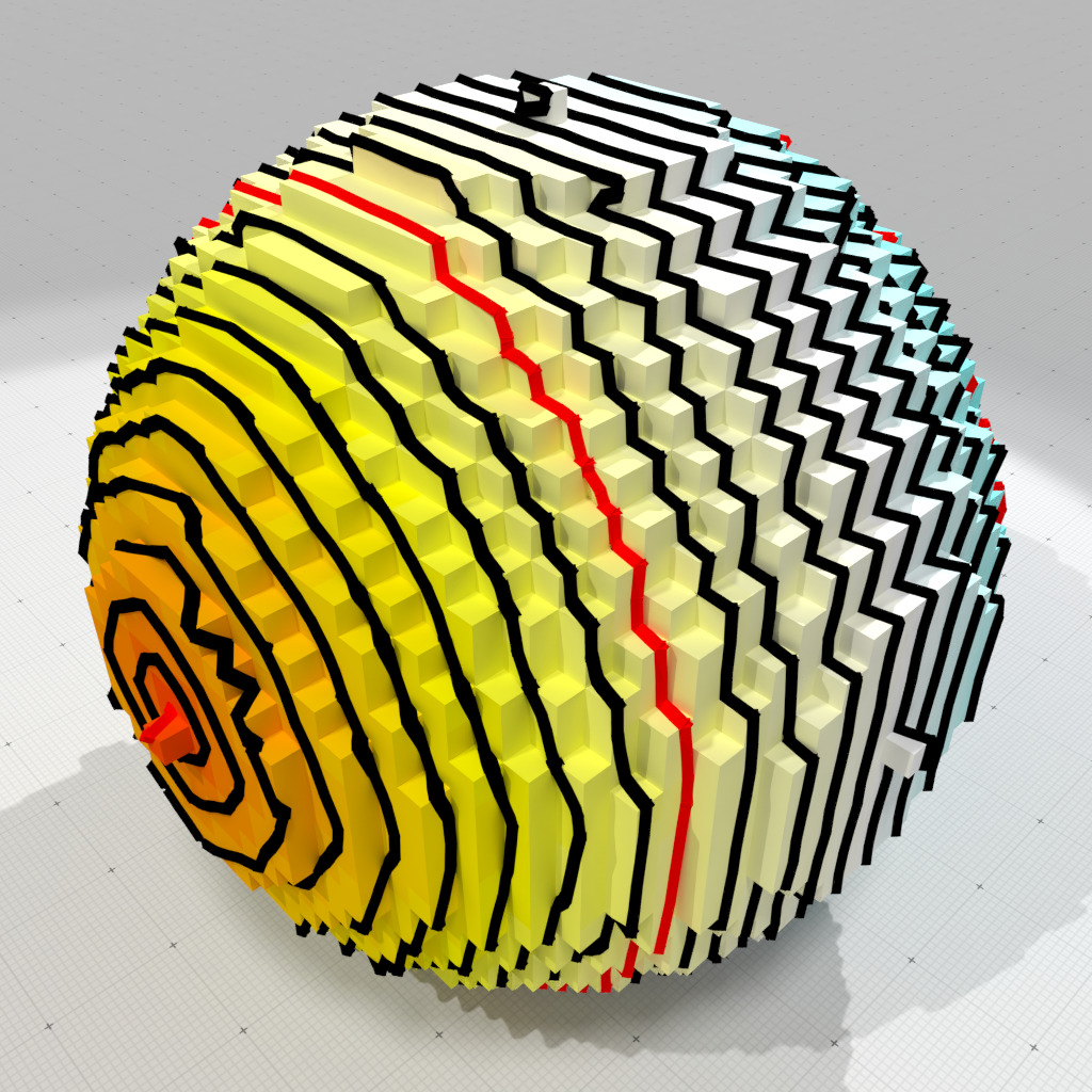
Exact geodesic distances on unit sphere digitized at h=0.0625 (max d=3.02389)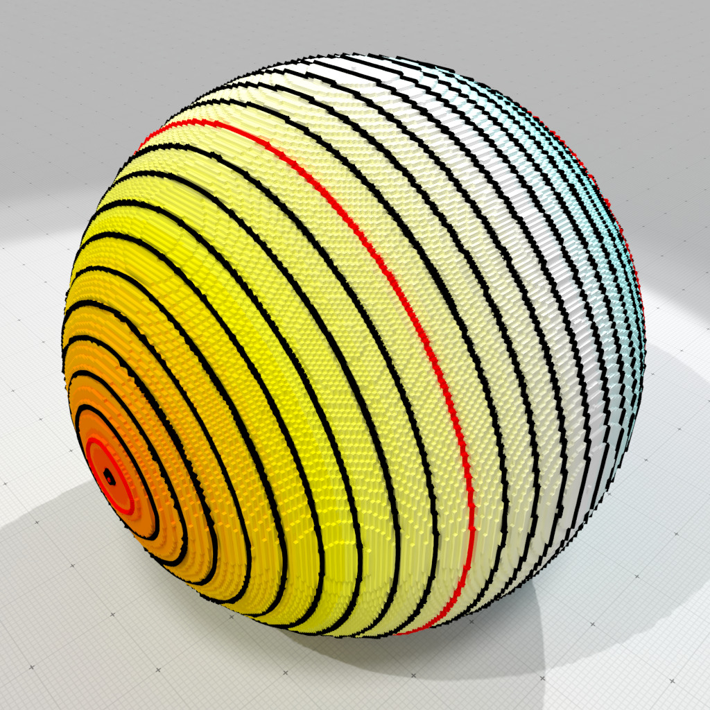

Approximate geodesic distances on unit sphere digitized at h=0.01 (max d=3.1269)

Table of Contents