Digital surface regularization by normal vector alignment

Table of Contents

• Introduction
• Main usages
• Local control

Author(s) of this documentation:

David Coeurjolly

Part of the Geometry package.

This part of the manual describes classes and functions related to the regularization of digital surfaces: Given an input normal vector field attached to digital surface surfels, the regularization outputs a piecewise smooth quadrangulated surface such that each quad is as perpendicular as possible to the input normal vector field. For more details, please refer to [29] and [30].

Related example: geometry/surfaces/testDigitalSurfaceRegularization.cpp

Note

In opposition to the method described in Digital surface regularization using the Shrouds algorithm, this digital surface regularization method is not limited to closed surfaces and can process open digital surfaces. Furthermore, the optimized energy is convex and fewer iterations are needed to converge to the optimal position. The price to pay is the computation of an estimated normal vector field.

Introduction

If \(P\) denotes the vertices of the input digital surface, \(F\) the set of (quadrilateral) faces and \(n_f\) an estimated normal vector on the face \(f\), we want the quad surface vertex positions \(P^*\) that minimizes the following energy function:

\[\mathcal{E}(P) := \alpha \sum_{i=1}^{n} \|p_i - \hat{p}_i\|^2 + \beta \sum_{f\in F} \sum_{{e_j} \in \partial{f} } ( e_j \cdot n_{f} )^2 + \gamma \sum_{i=1}^{n} \|\hat{p}_i - \hat{b}_i\|^2\,.\]

where \("\cdot"\) is the standard \(\mathbb{R}^3\) scalar product, \(e_j\in \partial{f}\) is an edge of the face \(f\) (and is equal to some \(p_k - p_l\)) and \( \hat{b}_i\) is the barycenter of the vertices adjacent to \(\hat{p}_i\).

The energy function is convex and can be minimized by solving a linear system as described in [29]. This minimization scheme is available in the DGtalTools (see volSurfaceRegularization). In this implementation, we consider an iterative scheme (gradient descent strategy) which allows us a finer control of the process.

Main usages

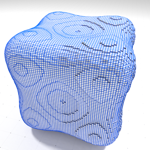
Starting from an implicit digital surface:

  typedef Shortcuts<Z3i::KSpace> SH3;
  typedef ShortcutsGeometry<Z3i::KSpace> SHG3;
  auto params = SH3::defaultParameters()
  | SHG3::defaultParameters();
  
  params( "polynomial", "goursat" )( "gridstep", 1.0)("verbose", 0);
  auto implicit_shape  = SH3::makeImplicitShape3D  ( params );
  auto digitized_shape = SH3::makeDigitizedImplicitShape3D( implicit_shape, params );
  auto K               = SH3::getKSpace( params );

with the following geometry (with a gridstep set to 0.3):

Input digital surface.

The regularization class instance can be set up using the following syntax:

    auto surface         = SH3::makeDigitalSurface( digitized_shape, K, params );
    auto surfels         = SH3::getSurfelRange( surface, params );
    DigitalSurfaceRegularization<SH3::DigitalSurface> regul(surface);
    regul.init();
    regul.attachConvolvedTrivialNormalVectors(params);

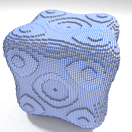
The DigitalSurfaceRegularization::init() method sets some default values for the \(\alpha\), \(\beta\) and \(\gamma\) parameters. Such parameters can be either chosen as global values (e.g. init(alpha,beta,gamma)), or as local weights. In the latter case, the user must specify a vector of \(\alpha[i]\), \(\beta[i]\) and \(\gamma[i]\) values, one per digital surface pointels (see Local control). In this example, the normal vector field attached to the surfels is a trivial normal estimator whose normals are given by local convolution of input quad normals. We can now minimize the energy as follows:

    auto finalenergy = regul.regularize();

Note that the user can specify the number of steps of the gradient descent as well as the initial learning rate. Note that if the DigitalSurfaceRegularization::regularize() method is called another time, the descent starts from the previous results (aka warm restart). Using the default settings (and the trivial normal vectors), we obtain the following reconstruction.

Regularized digital surface (trivial normal vectors).

Note

The regularized position can be retrieved using the getREgularizedPosition() method. E.g.

    auto regularizedPosition = regul.getRegularizedPositions();
    auto original  = regul.getOriginalPositions();

Warning

At this point, the digital surface must be closed.

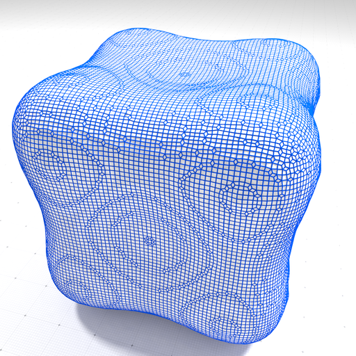
A key ingredient of the approach is to be able to change the input normal bundle. One can consider normal vectors from Integral invariant curvature estimator 2D/3D. Normal vectors can be attached using either a functor, a function or a lambda. For example, using Shortcuts (for the impatient developper)

    auto ii_normals = SHG3::getIINormalVectors(digitized_shape, surfels, params);
    DigitalSurfaceRegularization<SH3::DigitalSurface> regul(surface);
    regul.init();
    auto surfelIndex = regul.getSurfelIndex();
    regul.attachNormalVectors([&](SH3::SCell &c){ return ii_normals[ surfelIndex[c] ];} );

to obtain

Regularized digital surface (II normal vectors).

For piecewise smooth reconstruction, one can consider preprocessing of the normal vector field using Piecewise-smooth approximation using a discrete calculus model of Ambrosio-Tortorelli functional

Local control

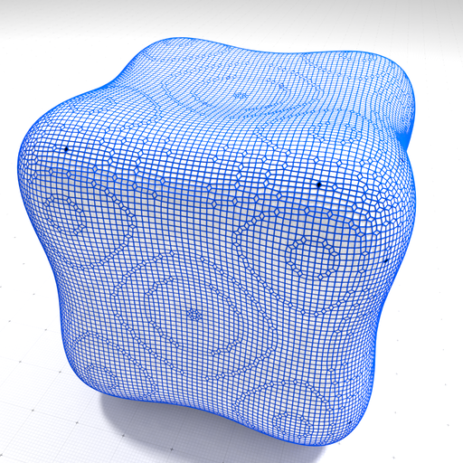
As discussed above, the user can control the weights \(\alpha\), \(\beta\) and \(\gamma\) per digital surface vertex. For instance using the following weights:

    DigitalSurfaceRegularization<SH3::DigitalSurface> regul3(surface);
    for(auto i = 0 ; i < original.size(); ++i)
      if (original[i][0]<0.0)
      {
        alphas[i] = 4.0;
        betas[i]  = 0.0000001;
        gammas[i] = 0.0;
      }
    regul3.init(alphas,betas,gammas);
    regul3.attachConvolvedTrivialNormalVectors(params);
    energybis = regul3.regularize();

we obtain a regularization with a locally adapted data attachment term.

Regularization with local data attachment weight.