This part of the manual describes how to visualize 3D objects and how to import them from binary file (.obj or pgm3d)
Display3D: a stream mechanism from abstract class Display3D
The semi-abstract template class Display3D defines the stream mechanism to display 3d primitive (like PointVector, DigitalSetBySTLSet, Object ...). The PolyscopeViewer class permits an interactive visualization (based on Polyscope (OpenGL backend)).
Display3D have two template parameters which correspond to the digital space and the Khalimsky space used to put the figures. From the Digital Space and Khalimsky Space, we use the associated embedding mechanism to convert digital objects to structures in \( \mathbb{R}^n\).
- Warning
- Do not forget to enable Polyscope at the cmake step, e.g. with cmake .. -DGTAL_WITH_POLYSCOPE_VIEWER=true.
Interactive visualization from PolyscopeViewer
The class PolyscopeViewer is a wrapper around the Polyscope library ( https://polyscope.run ).
It permits displaying geometrical data such as Point, Lines and (volumetric) meshes. The library handles 3D scenes movement and allows to attributes of displayed objects (such as colors and colormaps). The graphical interface is based on ImGUI (https://github.com/ocornut/imgui) which can be further extended.
First to use the PolyscopeViewer stream, you need to include the following headers:
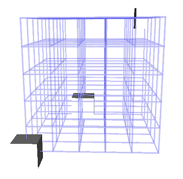
The following code snippet defines three points and a rectangular domain in Z3. It then displays them in a PolyscopeViewer object. The full code is in viewer3D-1-points.cpp.
The first step to draw objects is to create an instance of the PolyscopeViewer class:
Then we can display some 3D primitives:
The show() method enters the visualization loop and should be call after all object are drawn with the viewer. You should obtain the following visualization:
Interactive change of rendering
Polyscope has its own default rendering settings. Many parameters can be changed either programatically or at runtime directly within the viewer. This includes camera parameters (up direction, far/near plane, ...), materials of objects, lighting and many more. See polyscope documentation for available options (https://polyscope.run).
- Note
- Some rendered image of this documentation may have altered parameters to improve visibility such as scene extents or transparency mode.
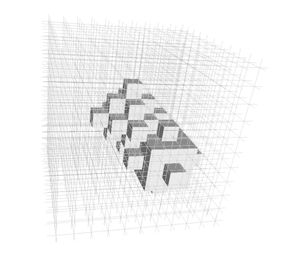
Visualization of DigitalSet and digital objects
The PolyscopeViewer class also allows to display directly a DigitalSet. The first step is to create a DigitalSet for example from the Shape class.
You should obtain the following visualization (see example: viewer3D-2-sets.cpp):
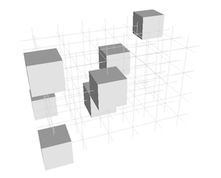
Drawmode selection: the example of digital objects in 3D
As for Board2D, a mode can be chosen to display elements. The viewer has several methods to adjust how objects are drawn.
or change the pair of adjacencies
You should obtain the two following visualizations (see example: viewer3D-3-objects.cpp):


Note that digital set was displayed with transparency by setting a custom color within the viewer.
Useful modes for several 3D drawable elements
Listing of different modes
As for Board2D the object can be displayed with different possible mode:
| Available modes | Description | Supported objects | Method |
|---|---|---|---|
| DEFAULT | Default rendering | Any | viewer.defaultStyle() |
| PAVING | Draws points as cubes | Point-based objects (Point, Domain, Object, DigitalSet, ...) | viewer.drawAsPaving() |
| BALL | Draws points as spheres | Point-based objects (Point, Domain, Object, DigitalSet, ...) | viewer.drawAsBalls() |
| GRID | Draws object with gridlines | Domains | viewer.drawAsGrid(true | false) |
| ADJACENCIES | Draws adjacencies relations | Objects | viewer.drawAdjacencies(true | false) |
| SIMPLIFIED | Draws quad instead of prism | 2D Signed KCells | viewer.drawAsSimplified(true | false) |
Examples with Objet modes
The file viewer3D-4-modes.cpp illustrates several possible modes to display these objects:
We can display the set of point and the domain
without mode change (see image (a)):
We can change the mode for displaying the domain (see image (b)):
(Note that to avoid transparency displaying artifacts, we need to display the domain after the voxel elements included in the domain)
It is also possible to change the mode for displaying the voxels: (see image (c))
(Note to enhance visibility, domain nodes are colored in black)
we obtain the following visualizations:


Changing the style for displaying drawable elements.
As for Board2D, it is possible to custom the way to display 3D elements. By default, the colors of elements are given by the viewer and can cycle through some of them. They can be changed directly in the user interface of the viewer. Colors can also be set programatically;
The example viewer3D-5-colors.cpp illustrates some possible customs :

If colors depend on values, please see section about adding properties to object instead of manually setting colors.
Adding clipping planes
It also possible through the stream mechanism to add a clipping plane thanks to the object ClippingPlane. We just have to add the real plane equation and add, as for displaying, an element. The file viewer3D-6-clipping.cpp gives a simple example.
From displaying a digital set defined from a Norm2 ball,
we can add, for instance, two different clipping planes:


It also possible to edit the clipping plane directly in the viewer (under View/Slice Planes) which allows to change colors, positions and if they are drawn or not.
Adding 2D image visualization in 3D
With the PolyscopeViewer class it is possible to display 2D slice image from a volume one. It can be done in a few steps (see example of viewer3D-8-2DSliceImages.cpp) :

Adding 3D image visualization
In the same way a 3D image can be displayed. By following the same stream operator, you will obtain such examples of display:
See more details in the example: io/viewers/viewer3D-9-3Dimages.cpp
Object names and groups
Each object that is drawn with the Display3D class is given a name as a string. This serves as a unique identifier and may also be used by viewers as user interface elements. It is possible to specify the name of an object with the draw function (internally, the stream operator will call this function).
In order to ensure uniqueness, the given may be altered if necessary. For example:
It is possible to specify where the counter will be placed with the "{i}" token (only first occurence is replaced). For KCell, the token "{d}" can also be used for dimension.
A common pattern when using the DGtal library is to iterate over a set of object, and then perform a computation and draw them (see tests/geometry/surfaces/testLocalConvolutionNormalVectorEstimator.cpp). However, this would imply having one object for each draw command, which can bloat the user interface and would make the viewer slow. It also limits the ability to have colormaps, since each value would be scattered across multiple objects. For this reason, a special variable can be set:
This will group new objects into the current list. However, this might fail if rendered objects change types (eg. alternating drawing lines and points). Therefore, the lists where the new objects should be pushed must be set manually with:
Adding quantities to objects
The class Display3D supports adding properties to objects. These properties can be colors, scalar values or vector information. These can be useful to display curvature information and/or computed normals. There are two ways to add these quantities. The first one is with the stream API, which is most useful for quick display of a couple of quantities:
The second approach, as powerful as the first one, requires the name of the object, but is more comfortable when the quantities are obtained after drawing.
Both methods can be used together and within loops:
These properties can be shown or hidden and their appearance modified directly in the graphical user interface.

It is also possible to add a last parameter to WithQuantity and addQuantity which is the element targeted by the quantity. For example, for a surface mesh, we may want to set the quantities at the vertices rather than on the faces when solving PDEs. However, the correct numbers of values should be supplied (eg. one per vertex and not one per face). Unfortunately, not every combination is supported (see table below). By default, it will use the scale corresponding to the dimension of the element (ie. right-most side in the "Supported Scale" column).
| Geometric display | Supported Scale | Name | DGtal object examples |
|---|---|---|---|
| Point | VERTEX | QuantityScale::VERTEX | (Real)Points in BALL mode, dim 0 KCell |
| Lines | VERTEX / EDGE | QuantityScale::VERTEX, QuantityScale::EDGE | Adjacencies, dim 1 KCell |
| Surface mesh | VERTEX / EDGE (Scalar)/ FACE | QuantityScale::VERTEX, QuantityScale::EDGE (Scalar), QuantityScale::FACE | dim 2 KCell in simplified mode |
| Volume mesh | VERTEX / CELL | QuantityScale::VERTEX, QuantityScale::CELL | (Real)Points, Objects, Domains, dim 2/3 KCell |
Extending the viewer
The viewer supports extensions that allow us to interact with the viewer at runtime. By default, PolyscopeViewer shows what object is clicked; but one may want to add custom UI, or enhance displayed information when an element is clicked. For this purpose, it is possible to set a callback that will be triggered upon three events: attach (only once), UI and clicks.
A useful method is Display3D::renderNewData that renders to the screen any newly added data. Another method, Display3D::renderAll can be used to (re)render every object; but run-time settings might be lost.
For PolyscopeViewer, user inputs and UI are managed with ImGUI. Also note that the viewer displays "by default", the name of the clicked polyscope structure.
Adding other standard primitive
The viewer can also display other standard primitives, like ball using the polyscope steps. For instance, to display a set of ball with different radius, you can follows these steps: